Table of Contents

🕶️ Motivation

Many biology and medical procedures involve counting cells from images taken with a microscope. Counting cells reveals the concentration of bacteria and viruses and gives vital information on the progress of a disease.

To accomplish the counting, researchers painstakingly count the cells by hand with the assistance of a device called hemocytometer. This process is repetitive, tedious, and prone to errors.

What if we could automate the counting by using an intelligent deep learning algorithm instead?

In this blog post, I will walk you through how to use the IceVision library and train a state-of-the-art deep learning model with Fastai to count microalgae cells.

Did I mention that all the tools used in this project are completely open-source and free of charge? Yes! If you’re ready let’s begin.

⚙️ Installation

Throughout this post, we will make use a library known as IceVision - a computer vision-focused library built to work with Fastai. Let’s install them first.

There are many ways to accomplish the installation. For your convenience, I’ve prepared an installation script that simplifies the process into just a few lines of code.

To get started, let’s clone the Git repository by typing the following in your terminal:

git clone https://github.com/dnth/microalgae-cell-counter-blogpost

Next, navigate into the directory:

cd microalgae-cell-counter-blogpost/

Install IceVision and all other libraries used for this post:

bash icevision_install.sh cuda11 0.12.0

Depending on your system CUDA version, you may want to change cuda11 to cuda10, especially on older systems. The number following the CUDA version is the version of IceVision. The version I’m using for this blog post is 0.12.0. You can alternatively replace the version number with master to install the bleeding edge version of IceVision from the master branch on Github.

If you would like to install the CPU version of the library it can be done with:

bash icevision_install.sh cpu 0.12.0

The installation may take a few minutes depending on your internet connection speed. Let the installation complete before proceeding.

🔖 Labeling the data

All deep learning models require data to work. To construct a model for microalgae cell counting, we require images of microalgae cells to work with. For the purpose of this post, I’ve acquired image samples from a lab.

The following shows a sample image of the microalgae cells as seen through a microscope. The cells are colored green.

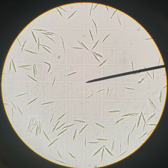
There are a bunch of other images in the data/not_labeled/ folder.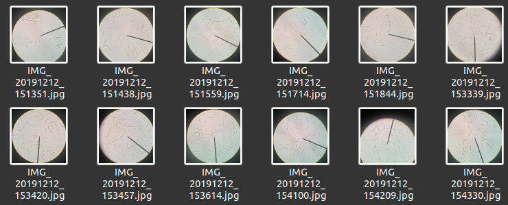

There is only one issue now, and that is the images are not labeled. Let’s label the images with bounding boxes using an open-source image labeling tool labelImg.

The labelImg app enables us to label images with class names and bounding boxes surrounding the object of interest. The following figure shows a demo of the app.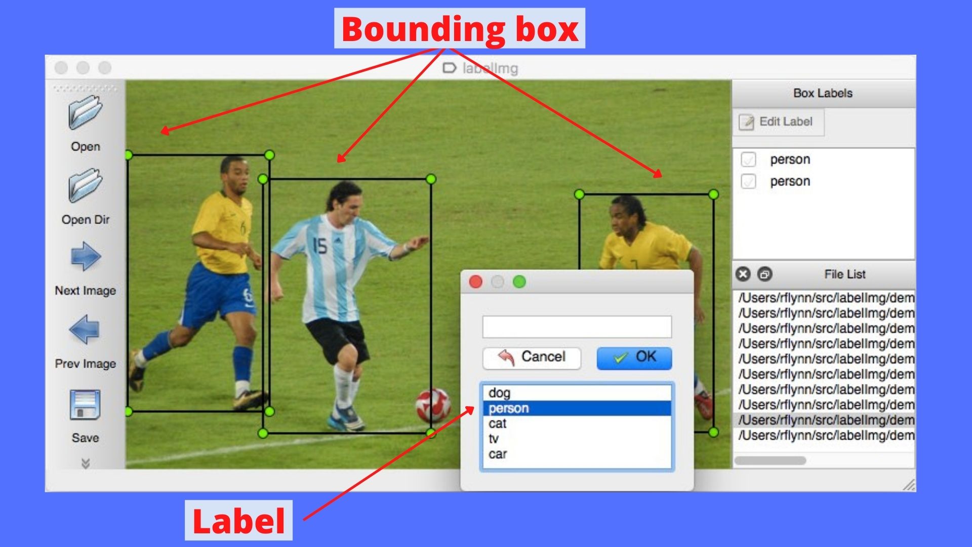

The labelImg app is already installed in the installation step. To launch the app, type in your terminal:

labelImg

A window like the following should appear.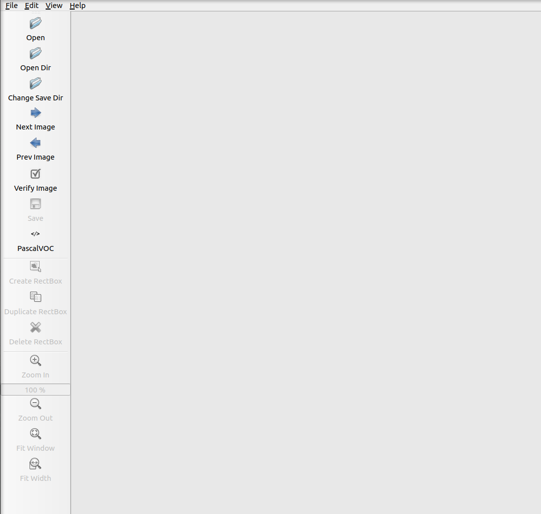

Let’s load the data/not_labeled/ images folder into labelImg and start labeling them! To do that, click on the Open Dir icon and navigate to the folder.

An image should now show up in labelImg. To label, click on the Create RectBox icon to start drawing bounding boxes around the microalgae cells. Next, you will be prompted to enter a label name. Key in microalgae as the label name. Once done, a rectangular bounding box should appear on-screen.

Now comes the repetitive part, we will need to draw a bounding box for each microalgae cell for all images in the folder. To accelerate the process I highly recommend the use of hotkeys keys with labelImg. The hotkeys are shown below.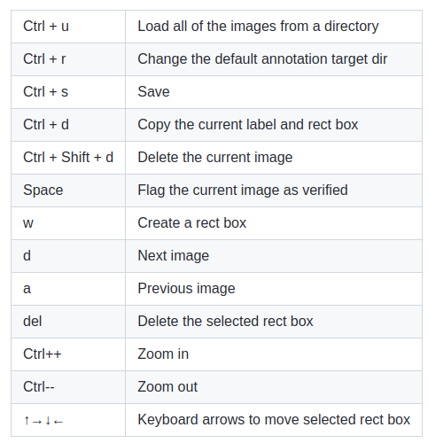

Once done, remember to save the annotations. The annotations are saved in an XML file with a file name matching to the image file name as shown below.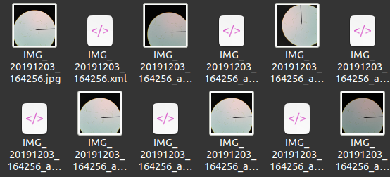

It took me a few hours to meticulously label the images. If you don’t feel like spending time labeling all the images (although I recommend doing them at least once), you can find the labeled ones in the data/labeled/ folder.

🌀 Modeling

Once the labeling is done, we are now ready to start modeling in a jupyter notebook environment.

To launch the jupyter notebook run the following in your terminal

jupyter lab

A browser window should pop up. On the left pane, double click the train.ipynb to open the notebook. All the codes in this section are inside the notebook. Here, I will attempt to walk you through just enough details of the code to get you started with modeling on your own data. If you require further clarifications, the IceVision documentation is a good starting point. Or drop me a message.

The first cell in the notebook is the imports. With IceVision all the necessary components are imported with one line of code:

from icevision.all import *

If something wasn’t properly installed, the imports will raise an error message. In that event, you must go back to the installation step before proceeding. If there are no errors, we are ready to dive in further.

🎯 Preparing datasets

After the imports, we must now load the labeled images and bounding boxes into jupyter. This is also known as data parsing and is accomplished with the following:

parser = parsers.VOCBBoxParser(annotations_dir="data/labeled", images_dir="data/labeled")

The parameter annotations_dir and images_dir are the directories to the images and annotations respectively. Since both the images and annotations are located in the same directory, they are the same as such in the code.

Next, we will randomly pick and divide the images and bounding boxes into two groups of data namely train_records and valid_records. By default, the split will be 80:20 to train:valid proportion. You can change the ratio by altering the values in RandomSplitter.

train_records, valid_records = parser.parse(data_splitter=RandomSplitter([0.8, 0.2])

The following code shows the class names from the parsed data:

parser.class_map

It should output:

<ClassMap: {'background': 0, 'Microalgae': 1}>

which shows a ClassMap that contains the class name as the key and class index as the value in a Python dictionary. The background class is automatically added. In the data labeling step, we do not need to label the background.

Next, we will apply basic data augmentation which is a technique used to diversify the training images by applying the random transformation. Learn more here.

The following code specifies the kinds of transformations we would like to perform on our images. Behind the scenes, these transformations are performed with the Albumentations library.

image_size = 640
train_tfms = tfms.A.Adapter([*tfms.A.aug_tfms(size=image_size, presize=image_size+128), tfms.A.Normalize()])
valid_tfms = tfms.A.Adapter([*tfms.A.resize_and_pad(image_size), tfms.A.Normalize()])

We must specify the dimensions of the image in image_size = 640. This value will then be used in tfms.A.aug_tfms that ensures that all images are resized to a 640x640 resolution and normalized in tfms.A.Normalize().

Some models like EfficientDet only work with image size divisible by 128. Other common values you can try are 384, 512, 768, etc. But beware using a large image size may consume more memory and in some cases halts training. Starting with a small value like 384 is probably a good idea. I found 640 works best for this dataset.

Use tfms.A.aug_tfms performs transformations to the image such as varying the lighting, rotation, shifting, flipping, blurring, padding, etc. The full list of transforms and the parameters can be found in the aug_tfms documentation.

In this code snippet, we created two distinct transforms namely train_tfms and valid_tfms that will be used during the training and validation steps respectively.

Next, we will apply the train_tfms to our train_records and valid_tfms to valid_records with the following snippet.

train_ds = Dataset(train_records, train_tfms)
valid_ds = Dataset(valid_records, valid_tfms)

This results in the creation of a Dataset object which is a collection of transformed images and bounding boxes.

To visualize the train_ds we can run:

samples = [train_ds[0] for _ in range(4)]
show_samples(samples, ncols=4)

This will show us 4 samples from the train_ds. Note the variations in lighting, translation, and rotation compared to the original images.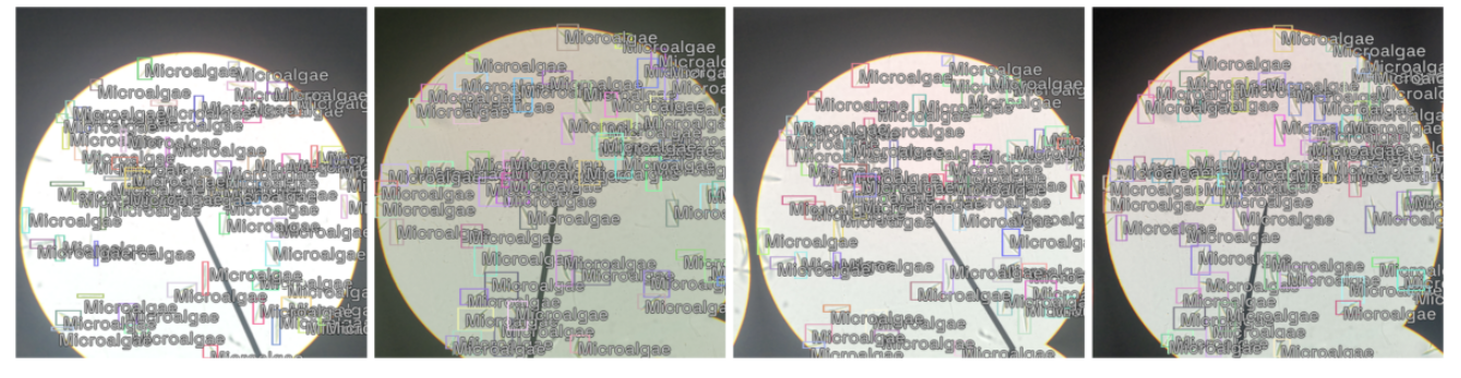

The transformations are applied on the fly. So each run on the snippet produces slightly different results.

🗝️ Choosing a library, model, and backbone

IceVision supports hundreds of high-quality pre-trained models from Torchvision, Open MMLab’s MMDetection, Ultralytic’s YOLOv5 and Ross Wightman’s EfficientDet.

Depending on your preference, you may choose the model and backbone from these libraries. In this post I will choose the VarifocalNet (VFNet) model from MMDetection which can be accomplished with:

model_type = models.mmdet.vfnet
backbone = model_type.backbones.resnet50_fpn_mstrain_2x
model = model_type.model(backbone=backbone(pretrained=True), num_classes=len(parser.class_map)) 

There are various ResNet backbones that you can select from such as resnet50_fpn_1x, resnet50_fpn_mstrain_2x, resnet50_fpn_mdconv_c3_c5_mstrain_2x, resnet101_fpn_1x, resnet101_fpn_mstrain_2x, resnet101_fpn_mdconv_c3_c5_mstrain_2x, resnext101_32x4d_fpn_mdconv_c3_c5_mstrain_2x, and resnext101_64x4d_fpn_mdconv_c3_c5_mstrain_2x.

Additionally, IceVision also recently supports state-of-the-art Swin Transformer backbone for the VFNet model swin_t_p4_w7_fpn_1x_coco, swin_s_p4_w7_fpn_1x_coco, and swin_b_p4_w7_fpn_1x_coco.

Which combination of model_type and backbone that performs best is something you need to experiment with. Feel free to experiment and swap out the backbone and note the performance of the model. There are other model types with their respective backbones which you can find here.

🏃 Metrics and Training

To start the training, the model needs to take in the images and bounding boxes from the train_ds and valid_ds we created.

For that, we will need to use a dataloader which will help us iterate over the elements in the dataset we created and load them into the model. We will construct two separate dataloaders for train_ds and valid_ds respectively.

train_dl = model_type.train_dl(train_ds, batch_size=2, num_workers=4, shuffle=True)
valid_dl = model_type.valid_dl(valid_ds, batch_size=2, num_workers=4, shuffle=False)

Here, we can specify the batch_size parameter which is the number of images and bounding boxes given to the model in a single forward pass. The shuffle parameter specifies if you would like to randomly shuffle the order of the data. The num_workers parameter specifies how many sub-processes to use to load the data. Let’s keep it at 4 for now.

Next, we need to specify a measure of how well our model performs during training. This measure is specified using a metric - which involves using specific math equations to output a score that tells us if the model is improving or not during training. Some commonly used metrics include accuracy, error rate, F1 Score, etc. For object detection tasks the COCOMetric is commonly used. If you are interested this blog explains the math behind the metrics used for object detection.

Once the metric is defined, we can then load all three components - dataloaders, model, and metric into a Fastai Learner for training.

metrics = [COCOMetric(metric_type=COCOMetricType.bbox)]
learn = model_type.fastai.learner(dls=[train_dl, valid_dl], model=model, metrics=metrics)

With deep learning models, there are many hyperparameters that we can configure before we run the training. One of the most important hyperparameters to get right is the learning rate. Since IceVision is built to work with Fastai, we have access to a handy tool known as the learning rate finder first proposed by Leslie Smith and popularized by the Fastai community for its effectiveness. This is an incredibly simple yet powerful tool to find a range of optimal learning rate values that gives us the best training performance.

All we need to do is run:

learn.lr_find()

which outputs: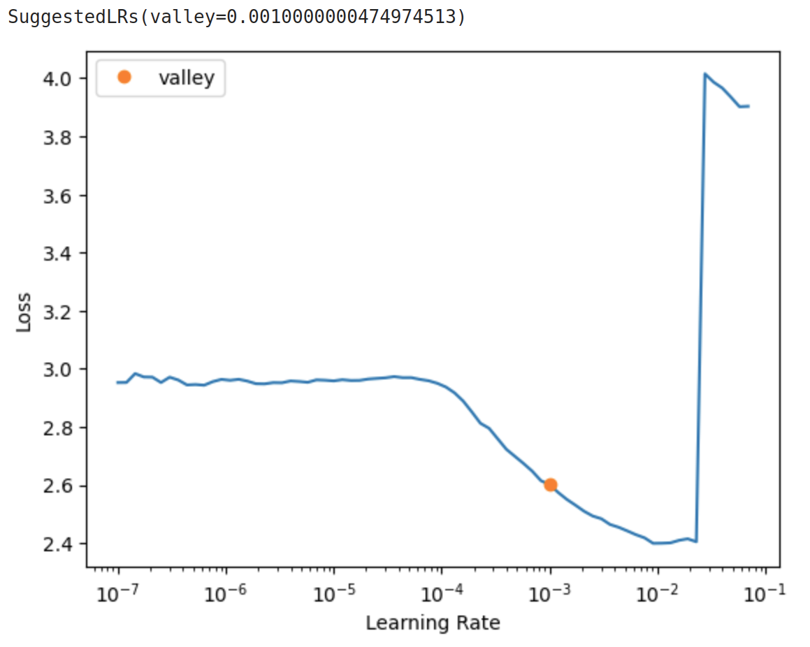

The most optimal learning rate value lies in the region where the loss descends most rapidly. From the figure above, this is somewhere in between 1e-4 to 1e-2. The orange dot on the plot shows the point where the slope is the steepest and is generally a good value to use as the learning rate.

Now, let’s load this learning rate value of 1e-3 into the fine_tune function and start training.

learn.fine_tune(10, 1e-3, freeze_epochs=1)

The first parameter in fine_tune is the number of epochs to train for. One epoch is defined as a complete iteration over the entire dataset. In this post, I will only train for 10 epochs. Training for longer will likely improve the model, so I will leave that to you to experiment with. The second parameter is the learning rate value we wish to use to train the model. Let’s put the value 1e-3 from the learning rate finder.

The above code snippet trains the model for 10 epochs. By default, this will start the training in two phases.

In the first phase ➀, only the last layer of the model is trained. The rest of the model is frozen. In the second phase ➁, the entire model is trained end-to-end. The figure below shows the training output.

The freeze_epochs parameter specifies the number of epochs to train in ➀.

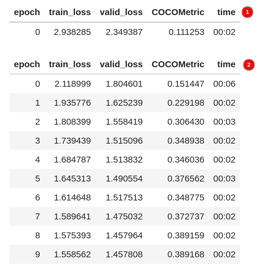
During the training, the train_loss, valid_loss, and COCOMetric are printed at every epoch. Ideally, the losses should decrease, and COCOMetric should increase the longer we train. As shown above, each epoch only took 2 seconds to complete on a GPU - which is incredibly fast.

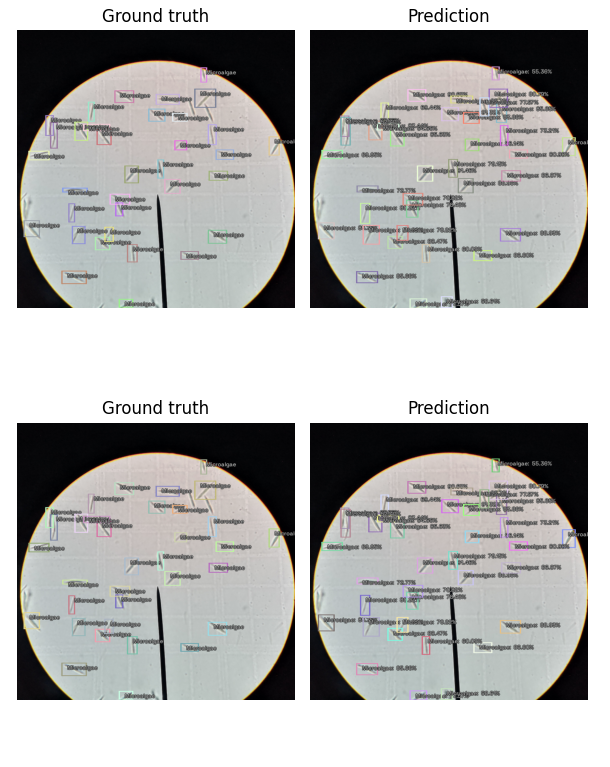
Once the training completes, we can view the performance of the model by showing the inference results on valid_ds. The following figure shows the output at a detection threshold of 0.5. You can increase the detection_threshold value to only show the bounding boxes with a higher confidence value.

model_type.show_results(model, valid_ds, detection_threshold=.5)

For completeness, here are the codes for the Modeling section which include steps to load the data, instantiate the model, train the model, and show the results. That’s only 17 lines of code!

 1
 2
 3
 4
 5
 6
 7
 8
 9
10
11
12
13
14
15
16
17
18
19
20
21
22
23
24

from icevision.all import *

parser = parsers.VOCBBoxParser(annotations_dir="data/labeled", images_dir="data/labeled")
train_records, valid_records = parser.parse()

image_size = 640
train_tfms = tfms.A.Adapter([*tfms.A.aug_tfms(size=image_size, presize=image_size+128), tfms.A.Normalize()])
valid_tfms = tfms.A.Adapter([*tfms.A.resize_and_pad(image_size), tfms.A.Normalize()])

train_ds = Dataset(train_records, train_tfms)
valid_ds = Dataset(valid_records, valid_tfms)

model_type = models.mmdet.vfnet
backbone = model_type.backbones.resnet50_fpn_mstrain_2x
model = model_type.model(backbone=backbone(pretrained=True), num_classes=len(parser.class_map)) 

train_dl = model_type.train_dl(train_ds, batch_size=2, num_workers=4, shuffle=True)
valid_dl = model_type.valid_dl(valid_ds, batch_size=2, num_workers=4, shuffle=False)

metrics = [COCOMetric(metric_type=COCOMetricType.bbox)]
learn = model_type.fastai.learner(dls=[train_dl, valid_dl], model=model, metrics=metrics)
learn.fine_tune(10, 1e-3, freeze_epochs=1)

model_type.show_results(model, valid_ds, detection_threshold=.5)

📨 Exporting model

Once you are satisfied with the performance and quality of the model, we can export all the model configurations (hyperparameters) and weights (parameters) for future use.

The following code packages the model into a checkpoint and exports it into a local directory.

from icevision.models.checkpoint import *
save_icevision_checkpoint(model,
                        model_name='mmdet.vfnet', 
                        backbone_name='resnet50_fpn_mstrain_2x',
                        img_size=640,
                        classes=parser.class_map.get_classes(),
                        filename='./models/model_checkpoint.pth',
                        meta={'icevision_version': '0.12.0'})

The parameters model_name, backbone_name, and img_size have to match what we used during training.

filename specifies the directory and name of the checkpoint file.

meta is an optional parameter you can use to save all other information about the model.

Once completed the checkpoint should be saved in the models/ folder. We can now use this checkpoint independently outside of the training notebook.

🧭 Inferencing on a new image

To demonstrate that the model checkpoint file can be loaded independently, I created another notebook with the name inference.ipynb. In this notebook, we are going to load the checkpoint and use it for inference on a brand new image.

Let’s import all the necessary packages:

from icevision.all import *
from icevision.models.checkpoint import *
from PIL import Image

And specify the checkpoint path.

checkpoint_path = "./models/model_checkpoint.pth"

We can load the checkpoint with the function model_from_checkpoint. From the checkpoint, we can retrieve all other configurations such as the model type, class map, image size, and the transforms.

checkpoint_and_model = model_from_checkpoint(checkpoint_path)
model = checkpoint_and_model["model"]
model_type = checkpoint_and_model["model_type"]
class_map = checkpoint_and_model["class_map"]
img_size = checkpoint_and_model["img_size"]
valid_tfms = tfms.A.Adapter([*tfms.A.resize_and_pad(img_size), tfms.A.Normalize()])

The model is now ready for inference. Let’s try to load an image with:

img = Image.open('data/not_labeled/IMG_20191203_164256.jpg')

We can pass the image into the end2end_detect function to run the inference.

pred_dict = model_type.end2end_detect(img, valid_tfms, model, 
                                      class_map=class_map, 
                                      detection_threshold=0.5,
                                      display_label=True, 
                                      display_bbox=True, 
                                      return_img=True, 
                                      font_size=50, 
                                      label_color="#FF59D6")

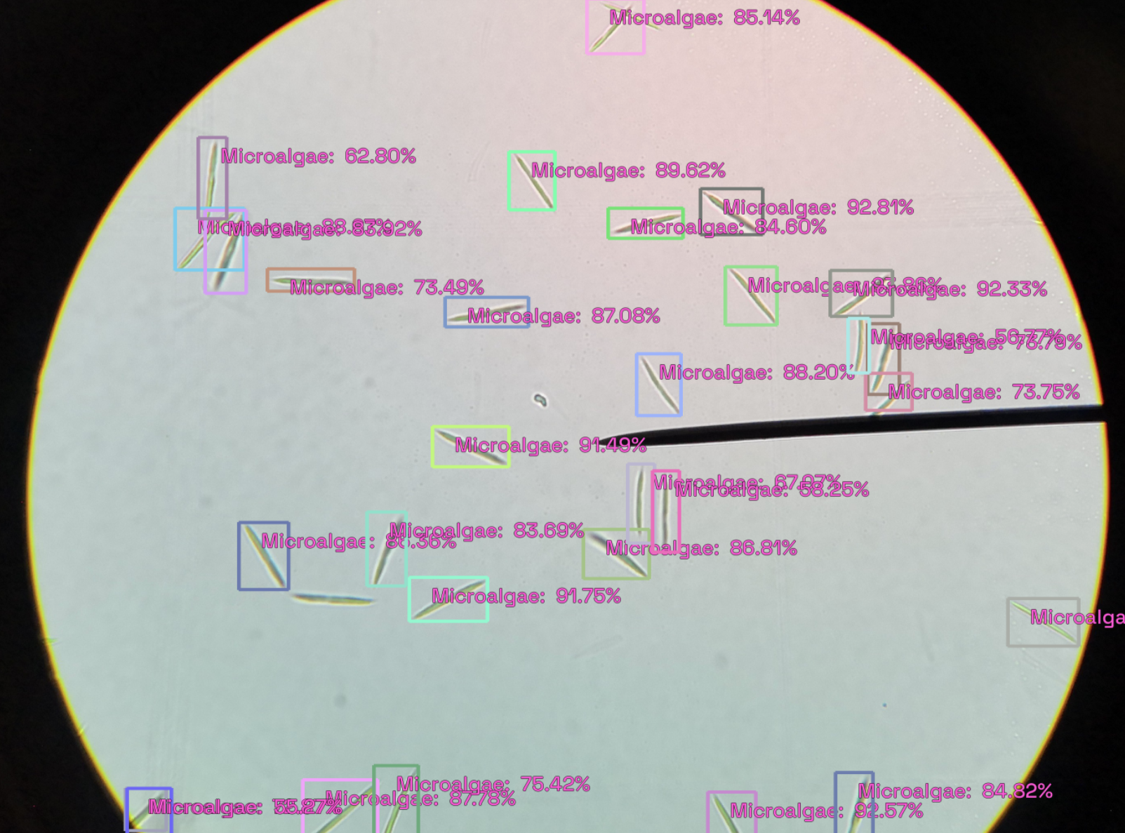
The output pred_dict is a Python dictionary. To view the output image with the bounding boxes:

pred_dict["img"]

which outputs

To count the number of microalgae cells on the image, we can count the number of bounding boxes on the image by with:

len(pred_dict['detection']['bboxes'])

which outputs 29 on my computer.

To save the image with the bounding boxes, you can run:

pred_dict["img"].save("inference.png")

As you can see, there are some missed detections of the microalgae cells. But, considering this is our first try, and we only trained for 10 epochs (which took less than 30 seconds to complete), this is an astonishing feat! Additionally, I’ve only used 17 labeled images to train the model.

In this post, I’ve demonstrated that we can train a sophisticated object detection model with only a few images in a very short time. This outstanding feat is possible thanks to the Fastai library which incorporated all the best practices in training deep learning models.

At this point, we have not even tuned any hyperparameters (other than learning rate) to optimize performance. Most hyperparameters are default values in Fastai that worked extremely well out-of-the-box with this dataset and model.

To improve performance, you may want to experiment by labeling more data and adjusting a few other hyperparameters such as image size, batch size, training epochs, the ratio of training/validation split, different model types, and backbones.

📖 Wrapping Up

Congratulations on making it through this post! It wasn’t that hard right? Hopefully, this post also boosted your confidence that object detection is not as hard as it used to be. With many high-level open-source packages like IceVision and Fastai, anyone with a computer and a little patience can break into object detection.

In this post, I’ve shown you how you can construct a model that detects microalgae cells.

In reality, the same steps can be used to detect any other cells or any other objects for that matter. Realizing this is an extremely powerful paradigm shift for me.

Think about all the problems we can solve by accurately detecting specific objects. Detecting intruders, detecting dangerous objects such as a gun, detecting defects on a production line, detecting smoke/fire, detecting skin cancer, detecting plant disease, and so much more.

Your creativity and imagination are the limits. The world is your oyster. Now go out there and use this newly found superpower to make a difference.

🙏 Comments & Feedback

If you find this useful, or if you have any questions, comments, or feedback, I would be grateful if you can leave them on the following Twitter post or drop me a message.

Sharing a blog post on how I trained a deep learning model to count microalgae cells in 17 lines of code with 17 labeled images using IceVision + @fastdotai #machinelearning #Microbiology #DataScientist #pythonprogramming #innovation #CellBiologyhttps://t.co/AcEtmLS0C9

— Dickson Neoh 🚀 (@dicksonneoh7) April 11, 2022

So what’s next? If you are interested to learn how I deploy this model on Android checkout this post.