Supercharging YOLOv5: How I Got 182.4 FPS Inference Without a GPU


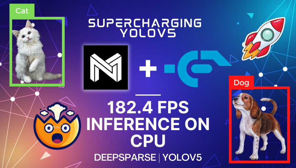
Table of Contents
🔥 Motivation
After months of searching, you’ve finally found the one.
The one object detection library that just works.
No installation hassle, no package version mismatch, and no CUDA errors.
I’m talking about the amazingly engineered YOLOv5 object detection library by Ultralytics.
Elated, you quickly find an interesting dataset from Roboflow and finally trained a state-of-the-art (SOTA) YOLOv5 model to detect firearms from image streams.
You ran through a quick checklist –
- Inference results, checked ✅
COCOmAP, checked ✅- Live inference latency, checked ✅
You’re on top of the world.
You can finally pitch the results to your clients next Monday. At the back of your mind, you can already see your clients’ impressed look on the astonishing feat.
On the pitching day, just when you thought things are going in the right direction. One of the clients asked,
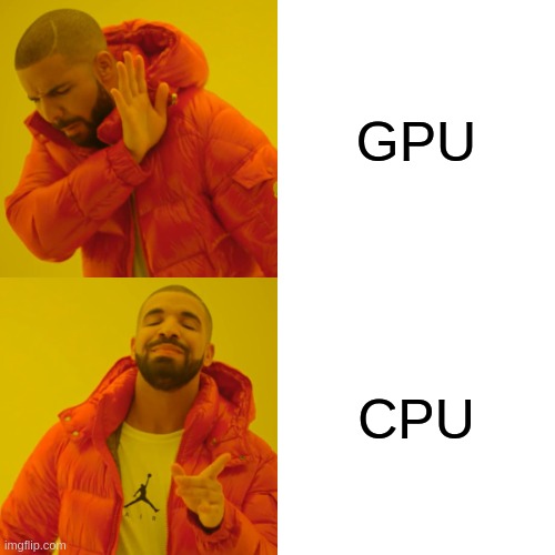
“Does your model run on our existing CPU?”
You flinched.
That wasn’t something you anticipated. You tried to convince them that GPUs are “the way forward” and it’s “the best way” to run your model in real-time.
You scanned the room and begin to notice the looks on their faces every time you said the word GPU and CPU.
Needless to say it didn’t go well. I hope nobody will have to face this awkward situation in a pitching session, ever. You don’t have to learn it the hard way, like I did.
You may wonder, can we really use consumer grade CPUs to run models in real-time?
🦾YES we can!
I wasn’t a believer, but now I am, after discovering Neural Magic.
In this post, I show you how you can supercharge your YOLOv5 inference performance running on CPUs using free and open-source tools by Neural Magic.
tip
By the end of this post, you will learn how to:
- Train a SOTA YOLOv5 model on your own data.
- Sparsify the model using SparseML quantization aware training, sparse transfer learning, and one-shot quantization.
- Export the sparsified model and run it using the DeepSparse engine at insane speeds.
P/S: The end result - YOLOv5 on CPU at 180+ FPS using only 4 CPU cores! 🚀
info
If you’re completely new to YOLOv5, get up to speed by reading this tutorial by Exxact.
If that sounds exciting let’s dive in 🧙
🔩 Setting Up
🔫 Dataset
The recent gun violence news had me thinking deeply about how we can prevent incidents like these again. This is the worst gun violence since 2012, and 21 innocent lives were lost.
I’m deeply saddened, and my heart goes out to all victims of the violence and their loved ones.
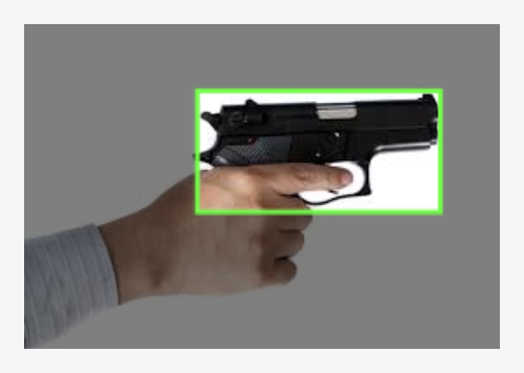
I’m not a lawmaker, so there is little I can do there. But, I think I know something in computer vision that might help. That’s when I came across the Pistols Dataset from Roboflow.
This dataset contains 2986 images and 3448 labels across a single annotation class: pistols. Images are wide-ranging: pistols in hand, cartoons, and staged studio-quality images of guns. The dataset was originally released by the University of Grenada.
🦸 Installation
Now let’s put the downloaded Pistols Dataset into the appropriate folder first.
I will put the downloaded images and labels into the datasets/ folder.
Let’s also put the sparsification recipes from SparseML into the recipes/ folder. More on recipes later.
Here’s a high-level overview of my directory.
├── req.txt
├── datasets
│   ├── pistols
│   │   ├── train
|   |   ├── valid
├── recipes
│   ├── yolov5s.pruned.md
│   ├── yolov5.transfer_learn_pruned.md
│   ├── yolov5.transfer_learn_pruned_quantized.md
|   └── ...
└── yolov5-train
        ├── data
        |   ├── hyps
        |   |   ├── hyps.scratch.yaml
        |   |   └── ...
        |   ├── pistols.yaml
        |   └── ...
        ├── models_v5.0
        |   ├── yolov5s.yaml
        |   └── ...
        ├── train.py
        ├── export.py
        ├── annotate.py
        └── ...
note
req.txt- Requirement file to install all packages used in this post.datasets/- Contains the train and validation images/labels downloaded from Roboflow.recipes/- Contains sparsification recipes from the SparseML repo.yolov5-train/- Cloned directory from Neural Magic’s YOLOv5 fork.
NOTE: You can explore further into the folder structure on my Github repo.
warning
IMPORTANT: The sparsification recipes will only work with Neural Magic’s YOLOv5 fork and will NOT WORK with the original YOLOv5 by Ultralytics.
For this post, we are going to use a forked version of the YOLOv5 library that will allow us to do custom optimizations in the upcoming section.
To install, all packages in this blog post, run the following commands
git clone https://github.com/dnth/yolov5-deepsparse-blogpost
cd yolov5-deepsparse-blogpost/
pip install torch==1.9.0 torchvision==0.10.0 --extra-index-url https://download.pytorch.org/whl/cu111
pip install -r req.txt
Or, if you’re just getting started, I’d recommend 👇
tip
🔥 Run everything in Colab with a notebook I made here.
⛳ Baseline Performance
🔦 PyTorch
Now that everything’s in place, let’s start by training a baseline model with no optimization.
For that, run the train.py script in the yolov5-train/ folder.
python train.py --cfg ./models_v5.0/yolov5s.yaml \
                --data pistols.yaml \
                --hyp data/hyps/hyp.scratch.yaml \
                --weights yolov5s.pt --img 416 --batch-size 64 \
                --optimizer SGD --epochs 240 \
                --project yolov5-deepsparse --name yolov5s-sgd
note
--cfg– Path to the configuration file which stores the model architecture.--data– Path to the.yamlfile that stores the details of the Pistols dataset.--hyp– Path to the.yamlfile that stores the training hyperparameter configurations.--weights– Path to a pretrained weight.--img– Input image size.--batch-size– Batch size used in training.--optimizer– Type of optimizer. Options includeSGD,Adam,AdamW.--epochs– Number of training epochs.--project– Wandb project name.--name– Wandb run id.
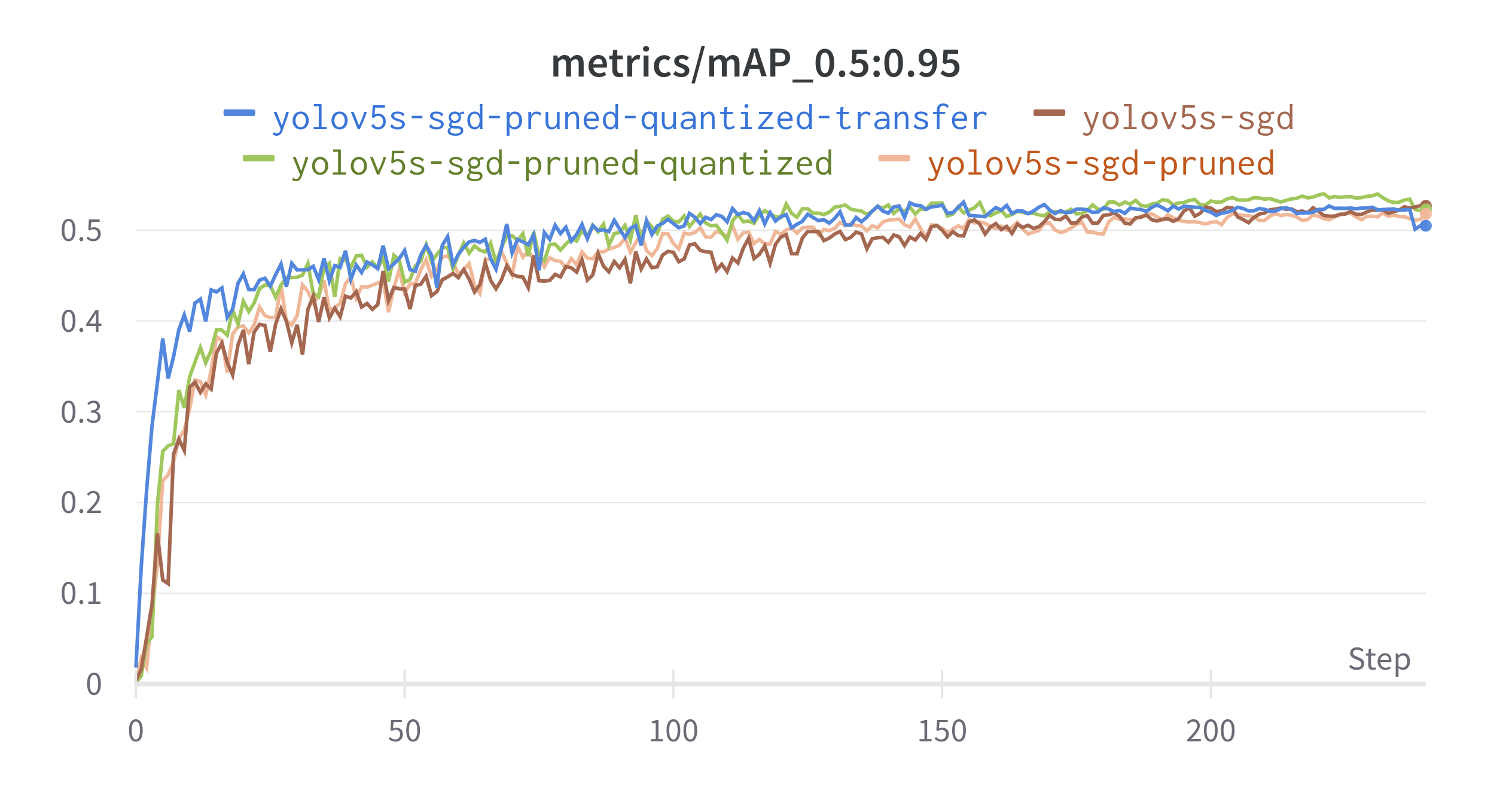
All metrics are logged to Weights & Biases (Wandb) here.
Once training’s done, let’s run inference on a video with the annotate.py script.
python annotate.py yolov5-deepsparse/yolov5s-sgd/weights/best.pt \
                --source data/pexels-cottonbro-8717592.mp4 \
                --engine torch \
                --image-shape 416 416 \
                --device cpu \
                --conf-thres 0.7
note
The first argument points to the .pt saved checkpoint.
--source- The input to run inference on. Options: path to video/images or just specify0to infer on your webcam.--engine- Which engine to use. Options:torch,deepsparse,onnxruntime.--image-size– Input resolution.--device– Device to use for inference. Options:cpuor0(GPU).--conf-thres– Confidence threshold for inference.
NOTE: The inference output will be saved in the annotation_results/ folder.
Here’s how it looks like running the baseline YOLOv5-S on an Intel i9-11900 using all 8 CPU cores.
- Average FPS : 21.91
- Average inference time (ms) : 45.58
Actually, the FPS looks quite decent already and might suit some applications even without further optimization.
But why settle when you can get something better? After all, that’s why you’re here, right? 😉
Meet 👇
🕸 DeepSparse Engine
DeepSparse is an inference engine by Neural Magic that runs optimally on CPUs. It’s incredibly easy to use. Just give it an ONNX model and you’re ready to roll.
Let’s export our .pt file into ONNX using the export.py script.
python export.py --weights yolov5-deepsparse/yolov5s-sgd/weights/best.pt \
                --include onnx \
                --imgsz 416 \
                --dynamic \
                --simplify
note
--weight – Path to the .pt checkpoint.
--include – Which format to export to. Options: torchscript, onnx, etc.
--imgsz – Image size.
--dynamic – Dynamic axes.
--simplify – Simplify the ONNX model.
And now, run the inference script again, this time using the deepsparse engine and with only 4 CPU cores in the --num-cores argument.
python annotate.py yolov5-deepsparse/yolov5s-sgd/weights/best.onnx \
        --source data/pexels-cottonbro-8717592.mp4 \
        --image-shape 416 416 \
        --conf-thres 0.7 \
        --engine deepsparse \
        --device cpu \
        --num-cores 4
- Average FPS : 29.48
- Average inference time (ms) : 33.91
Just like that, we improved the average FPS from 21+ (PyTorch engine on CPU using 8 cores) to 29+ FPS. All we did was use the ONNX model with the DeepSparse engine.
P/S: We are done with just the baselines here! The real action only happens next - when we run sparsification with 👇
👨🍳 SparseML and Recipes
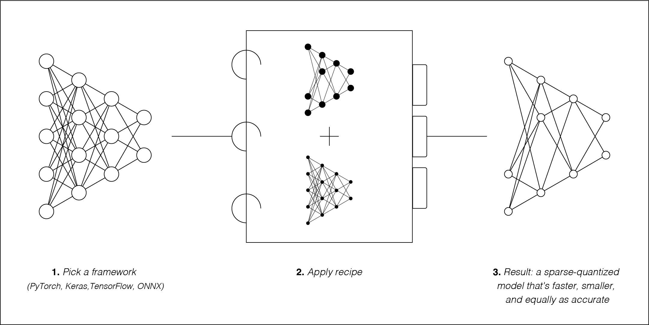
Image from SparseML documentation page.
Sparsification is the process of removing redundant information from a model. The result is a smaller and faster model.
This is how we speed up our YOLOv5 model, by a lot!
tip
In general, there are 2 methods to sparsify a model - Pruning and Quantization.
Pruning - Removing unused weights in the model.
Quantization - Forcing a model to use a less accurate storage format i.e. from 32-bit floating point (FP32) to 8-bit integer (INT8).
⚡ P/S: Used together or separately both pruning and quantization result in a smaller and faster model!
How do we sparsify models?
Using SparseML - an open-source library by Neural Magic. With SparseML you can sparsify neural networks by applying pre-made recipes to the model. You can also modify the recipes to suit your needs.
note
There are 3 methods to sparsify models with SparseML:
1️⃣ Post-training (One-shot).
2️⃣ Sparse Transfer Learning.
3️⃣ Training Aware.
NOTE: 1️⃣ does not require re-training but only supports dynamic quantization. 2️⃣ and 3️⃣ requires re-training and supports pruning and quantization which may give better results.
You may wonder, this sounds too good to be true!
What’s the caveat?
Good question!
With sparsification, you can expect a slight loss in accuracy depending on the degree of sparsification. Highly sparse models are usually less accurate than the original model but gains significant boost in speed and latency.
With the recipes from SparseML, the loss of accuracy ranges from 2% to 6%. In other words the recovery is 94% to 98% compared to the performance of the original model. In exchange, we gain phenomenal speedups, ranging from 2x to 10x faster!
In most situations, this is not a big deal. If the accuracy loss is something you can tolerate, then let’s sparsify some models already! 🤏.
☝️ One-Shot
The one-shot method is the easiest way to sparsify an existing model as it doesn’t require re-training.
But this only works well for dynamic quantization, for now. There are ongoing works in making one-shot work well for pruning.
Let’s run the one-shot method on the baseline model we trained earlier.
All you need to do is add a --one-shot argument to the training script, and specify a pruning --recipe.
Remember to specify --weights to the location of the best checkpoint from the training.
python train.py --cfg ./models_v5.0/yolov5s.yaml \
                --recipe ../recipes/yolov5s.pruned.md \
                --data pistols.yaml --hyp data/hyps/hyp.scratch.yaml \
                --weights yolov5-deepsparse/yolov5s-sgd/weights/best.pt \
                --img 416 --batch-size 64 --optimizer SGD --epochs 240 \
                --project yolov5-deepsparse --name yolov5s-sgd-one-shot \
                --one-shot
It should generate another .pt in the directory specified in --name.
This .pt file stores the quantized weights in int8 format instead of fp32 resulting in a reduction in model size and inference speedups.
Next, let’s export the quantized .pt file into ONNX format.
python export.py --weights yolov5-deepsparse/yolov5s-sgd-one-shot/weights/checkpoint-one-shot.pt \
                 --include onnx \
                 --imgsz 416 \
                 --dynamic \
                 --simplify
And run an inference
python annotate.py yolov5-deepsparse/yolov5s-sgd-one-shot/weights/checkpoint-one-shot.onnx \
                --source data/pexels-cottonbro-8717592.mp4 \
                --image-shape 416 416 \
                --conf-thres 0.7 \
                --engine deepsparse \
                --device cpu \
                --num-cores 4
- Average FPS : 32.00
- Average inference time (ms) : 31.24
At no re-training cost, we are performing 10 FPS better than the original model. We maxed out at about 40 FPS!
The one-shot method only took seconds to complete. If you’re looking for the easiest method for performance gain, one-shot is the way to go.
But, if you’re willing to re-train the model to double its performance and speed, read on 👇
🤹♂️ Sparse Transfer Learning
With SparseML you can take an already sparsified model (pruned and quantized) and fine-tune it on your own dataset. This is known as Sparse Transfer Learning.
This can be done by running
python train.py --data pistols.yaml --cfg ./models_v5.0/yolov5s.yaml
                --weights zoo:cv/detection/yolov5-s/pytorch/ultralytics/coco/pruned_quant-aggressive_94?recipe_type=transfer
                --img 416 --batch-size 64 --hyp data/hyps/hyp.scratch.yaml
                --recipe ../recipes/yolov5.transfer_learn_pruned_quantized.md
                --optimizer SGD
                --project yolov5-deepsparse --name yolov5s-sgd-pruned-quantized-transfer
The above command loads a sparse YOLOv5-S from Neural Magic’s SparseZoo and runs the training on your dataset.
The --weights argument points to a model from the SparseZoo.
There are more sparsified models available in SparseZoo.
I will leave it to you to explore which model works best.
Running inference with annotate.py results in
- Average FPS : 51.56
- Average inference time (ms) : 19.39
We almost 2x the FPS from the previous one-shot method!
Judging from the FPS value and mAP scores, Sparse Transfer Learning makes a lot of sense for most applications.
But, if you scrutinize further into the mAP metric on the Wandb dashboard, you’ll notice it’s slightly lower than the next method 💪.
✂ Pruned YOLOv5-S
Here, instead of taking an already sparsified model, we are going to sparsify our model by pruning it ourselves.
To do that we will use a pre-made recipe on the SparseML repo. This recipe tells the training script how to prune the model during training.
For that, we slightly modify the arguments of train.py
python train.py --cfg ./models_v5.0/yolov5s.yaml \
                --recipe ../recipes/yolov5s.pruned.md
                --data pistols.yaml \
                --hyp data/hyps/hyp.scratch.yaml \
                --weights yolov5s.pt --img 416
                --batch-size 64 --optimizer SGD \
                --project yolov5-deepsparse --name yolov5s-sgd-pruned
The only change here is the --recipe and the --name argument.
Also, there is no need to specify the --epoch argument because the number of training epochs is specified in the recipe.
--recipe tells the training script which recipe to use for the YOLOv5-S model.
In this case, we are using the yolov5s.pruned.md recipe which only prunes the model as it trains.
You can change how aggressive your model is pruned by modifying the yolov5s.pruned.md recipe.
warning
IMPORTANT: The sparsification recipes are model dependent. Eg. YOLOv5-S recipes will not work with YOLOv5-L.
So make sure you get the right recipe for the right model. Check out other YOLOv5 pre-made recipes here.
Running inference, we find
- Average FPS : 35.50
- Average inference time (ms) : 31.73
The drop in FPS is expected compared to the Sparse Transfer Learning method because this model is only pruned and not quantized.
But we gain higher mAP values.
🔬 Quantized YOLOv5-S
We’ve seen the effects of pruning, what about quantization? Let’s run quantization for the YOLOv5-S model and see how it behaves.
We could run the quantization without training (one-shot). But for better effects let’s train the model for 2 epochs. Re-training for 2 epochs allow the weights to re-adjust to the quantized values and hence produce better results.
The number of training epochs is specified in the yolov5s.quantized.md file.
Let’s run the train.py
python train.py --cfg ./models_v5.0/yolov5s.yaml \
                --recipe ../recipes/yolov5s.quantized.md \
                --data pistols.yaml \
                --hyp data/hyps/hyp.scratch.yaml \
                --weights yolov5-deepsparse/yolov5s-sgd/weights/best.pt --img 416 \
                --batch-size 64 --project yolov5-deepsparse --name yolov5s-sgd-quantized
Inferencing with annotate.py
- Average FPS : 43.29
- Average inference time (ms) : 23.09
We have a bump in the FPS compared to the pruned model.
With careful observation you’d notice a misdetection at the 0:03 second.
Here, we see that the quantized model is faster than the pruned model at the cost of detection accuracy. But note, in this model we’ve only trained for 2 epochs compared to 240 epochs with the pruned model. Re-training for longer may solve the misdetection issue.
We’ve seen how the YOLOv5-S model performs when it is
- Only pruned
- Only quantized
But, can we run both pruning and quantization?
Of course, why not? 🤖
🪚 Pruned + Quantized YOLOv5-S
Now, let’s take it to the next level by running both pruning and quantization.
Note the difference --recipe I’m using.
python train.py --cfg ./models_v5.0/yolov5s.yaml \
                --recipe ../recipes/yolov5.transfer_learn_pruned_quantized.md \
                --data pistols.yaml \
                --hyp data/hyps/hyp.scratch.yaml \
                --weights yolov5s.pt --img 416 \
                --batch-size 64 --optimizer SGD \
                --project yolov5-deepsparse --name yolov5s-sgd-pruned-quantized
Export with export.py and run inference with annotate.py.
We get
- Average FPS : 58.06
- Average inference time (ms) : 17.22
On our Wandb dashboard this model scores the highest mAP and is also the fastest.
It’s getting the best of both! 🎯
I wanted to end the post here. But there is still this nagging thought that I can’t ignore. It’s keeping me awake at night. So I had to do this 🤷♂️.
Every night I wonder how fast can we run YOLOv5 on CPUs? I mean the maximum possible FPS with SparseML + DeepSparse.
This led me to 👇
🚀 Supercharging with Smaller Models
In the YOLOv5 series, the YOLOv5-Nano is the smallest model of all. In theory, this should be the fastest.
So I’m putting my bets on this model. Let’s apply the same steps again with the YOLOv5-Nano model.
And
..
..
🚀🚀🚀
- Average FPS : 101.52
- Average inference time (ms) : 9.84
🤯 This is mindblowing! The max FPS hit the 180+ range. I never imagine these numbers are possible, especially using only 4 CPU cores.
Seeing this, I can now sleep peacefully at night 😴
🚧 Conclusion
What a journey this has been.
Gone are the days when we need GPUs to run models in real-time. With DeepSparse and SparseML, you can get GPU-class performance on commodity CPUs.
tip
In this post I’ve shown you how to:
- Train a SOTA YOLOv5 model with your own data.
- Sparsify the model using SparseML quantization aware training and one-shot quantization.
- Export the sparsified model and run it using the DeepSparse engine at insane speeds.
P/S: Check out codes on my GitHub repo.
If you ever get lost in the commands that I used for this post, fear not. I listed all commands I used to train all models on the README of the repo.
Also, feel to use the repo with your own dataset and give it a ⭐ if it helps your work.
If you enjoyed this post, you might also like the following post where I show how to accelerate your PyTorch Image Models (TIMM) 8x faster with ONNX Runtime and TensorRT.
Supercharge Your PyTorch Image Models: Bag of Tricks to 8x Faster Inference with ONNX Runtime & Optimizations
🙏 Comments & Feedback
I hope you’ve learned a thing or two from this blog post. If you have any questions, comments, or feedback, please leave them on the following Twitter/LinkedIn post or drop me a message.
Anyone can train a YOLOv5 (@ultralytics) nowadays. But deploying it on a CPU is such a PAIN.
— Dickson Neoh 🚀 (@dicksonneoh7) June 8, 2022
The pain ends here.
In this🧵 I'll show you how I got insane speeds (180+ FPS) running YOLOv5 on a consumer CPU using 4 only cores🤯
🔥 P/S: I use open-source tools by @neuralmagic. pic.twitter.com/b2vFOf57Ax
- GitHub
- Scholar
- Telegram
🤟 Follow me
Don't want to miss any of my future content? Follow me on Twitter and LinkedIn where I share these tips in bite-size posts.
🔄 Share this post
❤️ Show some love
Creating free ML contents doesn't pay my bills. Support me in creating more free contents like these. Consider buying me a coffee. Your support means a lot to me.