Supercharge Your PyTorch Image Models: Bag of Tricks to 8x Faster Inference with ONNX Runtime & Optimizations


Table of Contents
🚀 Motivation
Having real-time inference is crucial for computer vision applications. In some domains, a 1-second delay in inference could mean life or death.
Imagine sitting in a self-driving car and the car takes one full second to detect an oncoming speeding truck.
Just one second too late, and you could end up in the clouds 👼👼👼
Or if you’re lucky, you get a very up-close view of the pavement.

I hope that shows how crucial real-time inference is.
Thus, having real-time inference capability is paramount and will determine whether a model gets deployed or not. In many cases, you can pick one or the other:
- A fast model with low accuracy
- A slow model with high accuracy
But can we have the best of both worlds? I.e. a fast and accurate model?
That’s what this post is about.
tip
By the end of the post you’ll learn how to supercharge the inference speed of any image models from TIMM with optimized ONNX Runtime and TensorRT.
In short:
- 📥 Load any pre-trained model from TIMM.
- 🔄 Convert the model to ONNX format.
- 🖥️ Run inference with ONNX Runtime (CPU & CUDA Provider).
- 🎮 Run inference with TensorRT provider and optimized runtime parameters.
- 🧠 Bake the pre-processing into the ONNX model for faster inference.
You can find the code for this post on my GitHub repository here.
info
Are you non-technical?
Listen to this 10 mins conversation podcast that breaks down the content of this post in an ELI5 manner.
Note: Conversation generated using NotebookLM.
If you’re technical, and this sounds exciting, then let’s dive in! 🏊♂️
💻 Installation
Let’s begin with the installation.
I will be using a conda environment to install the packages required for this post. Feel free to the environment of your choice.
conda create -n supercharge_timm_tensorrt python=3.11
conda activate supercharge_timm_tensorrt
We’ll be using the timm library to load a pre-trained model and run inference. So let’s install timm.
pip install timm
At the time of writing, there are over 1370 models available in timm. Any of which can be used in this post.
🔧 Load and Infer
Let’s load a top performing model from the timm leaderboard - the eva02_large_patch14_448.mim_m38m_ft_in22k_in1k model.
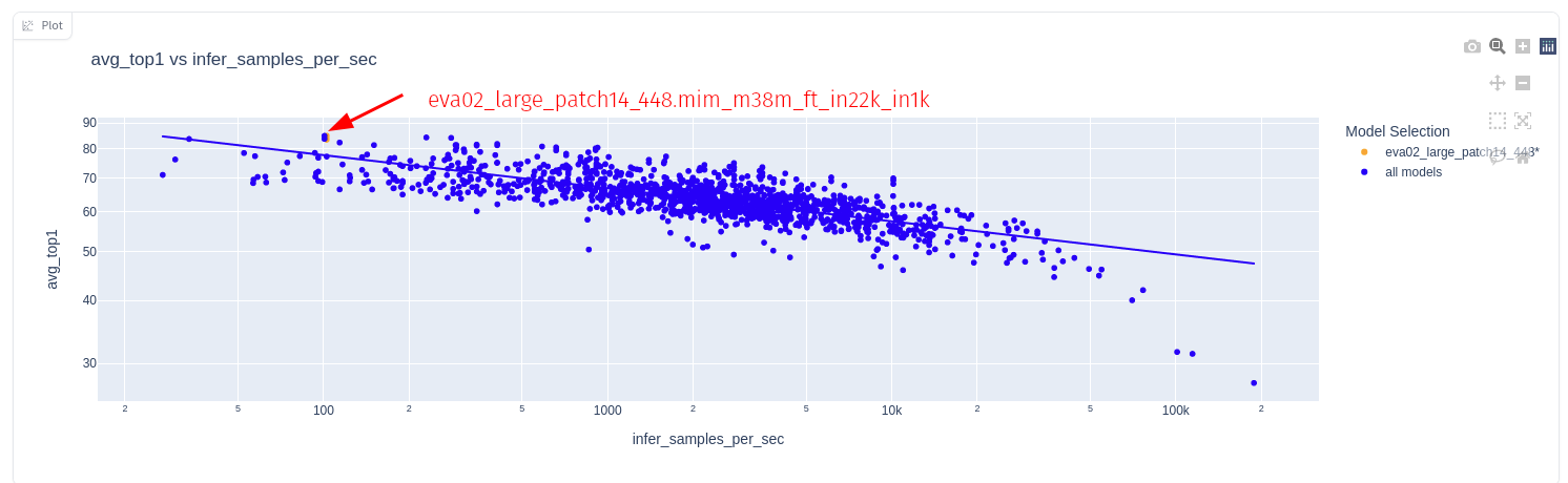
The plot above shows the accuracy vs inference speed for the EVA02 model.
Look closely, the EVA02 model achieves top ImageNet accuracy (90.05% top-1, 99.06% top-5) but is lags in speed.
Check out the model on the timm leaderboard here.
So let’s get the EVA02 model on our local machine
import timm

model_name = 'eva02_large_patch14_448.mim_m38m_ft_in22k_in1k'
model = timm.create_model(model_name, pretrained=True).eval()
Get the data config and transformations for the model
data_config = timm.data.resolve_model_data_config(model)
transforms = timm.data.create_transform(**data_config, is_training=False)
And run an inference to get the top 5 predictions
import torch
from PIL import Image
from urllib.request import urlopen

img = Image.open(urlopen('https://huggingface.co/datasets/huggingface/documentation-images/resolve/main/beignets-task-guide.png'))

with torch.inference_mode():
    output = model(transforms(img).unsqueeze(0))

top5_probabilities, top5_class_indices = torch.topk(output.softmax(dim=1) * 100, k=5)
Next, decode the predictions into class names as a sanity check
from imagenet_classes import IMAGENET2012_CLASSES

im_classes = list(IMAGENET2012_CLASSES.values())
class_names = [im_classes[i] for i in top5_class_indices[0]]

for name, prob in zip(class_names, top5_probabilities[0]):
    print(f"{name}: {prob:.2f}%")

Top 5 predictions:
- espresso: 26.78%
- eggnog: 2.88%
- cup: 2.60%
- chocolate sauce, chocolate syrup: 2.39%
- bakery, bakeshop, bakehouse: 1.48%
Looks like the model is doing it’s job.
Now let’s benchmark the inference latency.
⏱️ Baseline Latency
We will run the inference 10 times and average the inference time.
import time

def run_benchmark(model, device, num_images=10):
    model = model.to(device)

    with torch.inference_mode():
        start = time.perf_counter()
        for _ in range(num_images):
            input_tensor = transforms(img).unsqueeze(0).to(device)
            model(input_tensor)
        end = time.perf_counter()

    ms_per_image = (end - start) / num_images * 1000
    fps = num_images / (end - start)

    print(f"PyTorch model on {device}: {ms_per_image:.3f} ms per image, FPS: {fps:.2f}")
Let’s benchmark on CPU and GPU.
# CPU Benchmark
run_benchmark(model, torch.device("cpu"))

# GPU Benchmark
if torch.cuda.is_available():
    run_benchmark(model, torch.device("cuda"))
Alright the benchmarks are in
- PyTorch model on cpu: 1584.379 ms per image, FPS: 0.63
- PyTorch model on cuda: 77.226 ms per image, FPS: 12.95
Although the performance on the GPU is not bad, 12+ FPS is still not fast enough for real-time inference. On my reasonably modern CPU, it took over 1.5 seconds to run an inference.
Definitely not self-driving car material 🤷
note
I’m using the following hardware for the benchmarks:
- GPU - NVIDIA RTX 3090
- CPU - 11th Gen Intel® Core™ i9-11900 @ 2.50GHz × 16
Now let’s start to improve the inference time.
🔄 Convert to ONNX
ONNX is an open and interoperable format for deep learning models. It lets us deploy models across different frameworks and devices.
The key advantage of using ONNX is that it lets us deploy models across different frameworks and devices, and offers some performance gains.
To convert the model to ONNX format, let’s first install onnx.
pip install onnx
And export the model to ONNX format
import timm
import torch

model = timm.create_model(
    "eva02_large_patch14_448.mim_m38m_ft_in22k_in1k", pretrained=True
).eval()

onnx_filename = "eva02_large_patch14_448.onnx"

torch.onnx.export(
    model,
    torch.randn(1, 3, 448, 448),
    onnx_filename,
    export_params=True,
    opset_version=20,
    do_constant_folding=True,
    input_names=["input"],
    output_names=["output"],
    dynamic_axes={"input": {0: "batch_size"},
                  "output": {0: "batch_size"}},
)
note
Here are the descriptions for the arguments you can pass to the torch.onnx.export function:
| Parameter | Description |
|---|---|
torch.randn(1, 3, 448, 448) | A dummy input tensor with the appropriate shape |
export_params | Whether to export the model parameters |
do_constant_folding | Whether to do constant folding for optimization |
input_names | The name of the input node |
output_names | The name of the output node |
dynamic_axes | Dynamic axes for the input and output nodes |
If there are no errors, you will end up with a file called eva02_large_patch14_448.onnx in your working directory.
tip
Inspect and visualize the ONNX model using the Netron webapp.
🖥️ ONNX Runtime on CPU
To run the and inference on the ONNX model, we need to install onnxruntime. This is the ’engine’ that will run the ONNX model.
pip install onnxruntime
One (major) benefit of using ONNX Runtime is the ability to run the model without PyTorch as a dependency. This is great for deployment and for running inference in environments where PyTorch is not available.
The ONNX model we exported earlier only includes the model weights and the graph structure. It does not include the pre-processing transforms.
To run the inference using onnxruntime, we need to replicate the PyTorch transforms.
To find out the transforms that was used, you can print out the transforms.
print(transforms)
- Compose(
- Resize(size=(448, 448),
- interpolation=bicubic,
- max_size=None,
- antialias=True)
- CenterCrop(size=(448, 448))
- MaybeToTensor()
- Normalize(mean=tensor([0.4815, 0.4578, 0.4082]),
- std=tensor([0.2686, 0.2613, 0.2758]))
- )
Now let’s replicate the transforms using numpy.
def transforms_numpy(image: PIL.Image.Image):
    image = image.convert('RGB')
    image = image.resize((448, 448), Image.BICUBIC)
    img_numpy = np.array(image).astype(np.float32) / 255.0
    img_numpy = img_numpy.transpose(2, 0, 1)
    mean = np.array([0.485, 0.456, 0.406]).reshape(-1, 1, 1)
    std = np.array([0.229, 0.224, 0.225]).reshape(-1, 1, 1)
    img_numpy = (img_numpy - mean) / std
    img_numpy = np.expand_dims(img_numpy, axis=0)
    img_numpy = img_numpy.astype(np.float32)
    return img_numpy
Using the numpy, transforms let’s run inference with ONNX Runtime.
import onnxruntime as ort

# Create ONNX Runtime session with CPU provider
onnx_filename = "eva02_large_patch14_448.onnx"
session = ort.InferenceSession(
    onnx_filename,
    providers=["CPUExecutionProvider"] # Run on CPU
)

# Get input and output names
input_name = session.get_inputs()[0].name
output_name = session.get_outputs()[0].name

# Run inference
output = session.run([output_name],
                    {input_name: transforms_numpy(img)})[0]
If we inspect the output shape, we can see that it’s the same as the number of classes in the ImageNet dataset.
Let’s inspect the output.shape:
- (1, 1000)
And printing the top 5 predictions:
- espresso: 28.65%
- cup: 2.77%
- eggnog: 2.28%
- chocolate sauce, chocolate syrup: 2.13%
- bakery, bakeshop, bakehouse: 1.42%
We get the same results as the PyTorch model with ONNX Runtime. That’s a good sign!
Now let’s benchmark the inference latency on ONNX Runtime with a CPU provider (backend).
import time

num_images = 10
start = time.perf_counter()
for i in range(num_images):
    output = session.run([output_name], {input_name: transforms_numpy(img)})[0]
end = time.perf_counter()
time_taken = end - start

ms_per_image = time_taken / num_images * 1000
fps = num_images / time_taken

print(f"Onnxruntime CPU: {ms_per_image:.3f} ms per image, FPS: {fps:.2f}")
- Onnxruntime CPU: 2002.446 ms per image, FPS: 0.50
Ouch! That’s slower than the PyTorch model. What a bummer! It may seem like a step back, but we are only getting started.
Read on.
info
The remainder of this post assumes that you have a compatible NVDIA GPU. If you don’t, you can still use the CPU for inference by switch to the Intel OpenVINO or AMD backend.
There are more backends available including for mobile devices like Apple, Android, etc. Check them out here
These will be covered in a future post.
🖼️ ONNX Runtime on CUDA
Other than the CPU, ONNX Runtime offers other backends for inference. We can easily swap to a different backend by changing the provider. In this case we will use the CUDA backend.
To use the CUDA backend, we need to install the onnxruntime-gpu package.
warning
You must uninstall the onnxruntime package before installing the onnxruntime-gpu package.
Run the following to uninstall the onnxruntime package.
pip uninstall onnxruntime
Then install the onnxruntime-gpu package.
pip install onnxruntime-gpu==1.19.2
The onnxruntime-gpu package requires a compatible CUDA and cuDNN version. I’m running on onnxruntime-gpu==1.19.2 at the time of writing this post. This version is compatible with CUDA 12.x and cuDNN 9.x.
See the compatibility matrix here.
You can install all the CUDA dependencies using conda with the following command.
conda install -c nvidia cuda=12.2.2 \
                 cuda-tools=12.2.2 \
                 cuda-toolkit=12.2.2 \
                 cuda-version=12.2 \
                 cuda-command-line-tools=12.2.2 \
                 cuda-compiler=12.2.2 \
                 cuda-runtime=12.2.2
Once done, replace the CPU provider with the CUDA provider.
onnx_filename = "eva02_large_patch14_448.onnx"

session = ort.InferenceSession(
    onnx_filename,
    providers=["CUDAExecutionProvider"] # change the provider
)
The rest of the code is the same as the CPU inference.
Just with one line of code change, the benchmarks are as follows:
- Onnxruntime CUDA numpy transforms: 56.430 ms per image, FPS: 17.72
But that’s kinda expected. Running on the GPU, we should expect a speedup.
info
If you encounter the following error:
Failed to load library libonnxruntime_providers_cuda.so
with error: libcublasLt.so.12: cannot open shared object
file: No such file or directory
It means that the CUDA library is not in the library path. You need to export the library path to include the CUDA library.
export LD_LIBRARY_PATH="/home/dnth/mambaforge-pypy3/envs/supercharge_timm_tensorrt/lib:$LD_LIBRARY_PATH"
Replace the /home/dnth/mambaforge-pypy3/envs/supercharge_timm_tensorrt/lib with the path to your CUDA library.
Theres is one more trick we can use to squeeze out more performance - using CuPy for the transforms instead of NumPy.
CuPy is a library that lets us run NumPy code on the GPU. It’s a drop-in replacement for NumPy, so you can just replace numpy with cupy in your code and it will run on the GPU.
Let’s install CuPy compatible with our CUDA version.
pip install cupy-cuda12x
And we can use it to run the transforms.
def transforms_cupy(image: PIL.Image.Image):
    # Convert image to RGB and resize
    image = image.convert("RGB")
    image = image.resize((448, 448), Image.BICUBIC)

    # Convert to CuPy array and normalize
    img_cupy = cp.array(image, dtype=cp.float32) / 255.0
    img_cupy = img_cupy.transpose(2, 0, 1)

    # Apply mean and std normalization
    mean = cp.array([0.485, 0.456, 0.406], dtype=cp.float32).reshape(-1, 1, 1)
    std = cp.array([0.229, 0.224, 0.225], dtype=cp.float32).reshape(-1, 1, 1)
    img_cupy = (img_cupy - mean) / std

    # Add batch dimension
    img_cupy = cp.expand_dims(img_cupy, axis=0)

    return img_cupy
With CuPy, we got a tiny bit of performance improvement:
- Onnxruntime CUDA cupy transforms: 54.267 ms per image, FPS: 18.43
Using ONNX Runtime with CUDA is a little better than the PyTorch model on the GPU, but still not fast enough for real-time inference.
We have one more trick up our sleeve.
📊 ONNX Runtime on TensorRT
Similar to the CUDA provider, we have the TensorRT provider on ONNX Runtime. This lets us run the model using the TensorRT high performance inference engine by NVIDIA.
From the compatibility matrix, we can see that onnxruntime-gpu==1.19.2 is compatible with TensorRT 10.1.0.
To use the TensorRT provider, you need to have TensorRT installed on your system.
pip install tensorrt==10.1.0 \
            tensorrt-cu12==10.1.0 \
            tensorrt-cu12-bindings==10.1.0 \
            tensorrt-cu12-libs==10.1.0
Next you need to export library path to include the TensorRT library.
export LD_LIBRARY_PATH="/home/dnth/mambaforge-pypy3/envs/supercharge_timm_tensorrt/python3.11/site-packages/tensorrt_libs:$LD_LIBRARY_PATH"
Replace the /home/dnth/mambaforge-pypy3/envs/supercharge_timm_tensorrt/python3.11/site-packages/tensorrt_libs with the path to your TensorRT library.
Otherwise you’ll encounter the following error:
Failed to load library libonnxruntime_providers_tensorrt.so
with error: libnvinfer.so.10: cannot open shared object file:
No such file or directory
Next we need so set the TensorRT provider options in ONNX Runtime inference code.
providers = [
    (
        "TensorrtExecutionProvider",
        {
            "device_id": 0,
            "trt_max_workspace_size": 8589934592,
            "trt_fp16_enable": True,
            "trt_engine_cache_enable": True,
            "trt_engine_cache_path": "./trt_cache",
            "trt_force_sequential_engine_build": False,
            "trt_max_partition_iterations": 10000,
            "trt_min_subgraph_size": 1,
            "trt_builder_optimization_level": 5,
            "trt_timing_cache_enable": True,
        },
    ),
]

onnx_filename = "eva02_large_patch14_448.onnx"
session = ort.InferenceSession(onnx_filename, providers=providers)
The rest of the code is the same as the CUDA inference.
note
Here are the parameters and description for the TensorRT provider:
| Parameter | Description |
|---|---|
device_id | The GPU device ID to use. Using the first GPU in the system. |
trt_max_workspace_size | Maximum workspace size for TensorRT in bytes (8GB). Allows TensorRT to use up to 8GB of GPU memory for operations. |
trt_fp16_enable | Enables FP16 (half-precision) mode. Speeds up inference on supported GPUs while reducing memory usage. |
trt_engine_cache_enable | Enables caching of TensorRT engines. Speeds up subsequent runs by avoiding engine rebuilding. |
trt_engine_cache_path | Directory where TensorRT engine cache files will be stored. |
trt_force_sequential_engine_build | Allows parallel building of TensorRT engines for different subgraphs. |
trt_max_partition_iterations | Maximum number of iterations for TensorRT to attempt partitioning the graph. |
trt_min_subgraph_size | Minimum number of nodes required for a subgraph to be considered for conversion to TensorRT. |
trt_builder_optimization_level | Optimization level for the TensorRT builder. Level 5 is highest, can result in longer build times but potentially better performance. |
trt_timing_cache_enable | Enables timing cache. Helps speed up engine building by reusing layer timing information from previous builds. |
Refer to the TensorRT ExecutionProvider documentation for more details on the parameters.
And now let’s run the benchmark:
- TensorRT + numpy: 18.852 ms per image, FPS: 53.04
- TensorRT + cupy: 16.892 ms per image, FPS: 59.20
Running with TensorRT and cupy give us a 4.5x speedup over the PyTorch model on the GPU and 93x speedup over the PyTorch model on the CPU!
Thank you for reading this far. That’s the end of this post.
Or is it?
You could stop here and be happy with the results. After all we already got a 93x speedup over the PyTorch model.
But.. if you’re like me and you wonder how much more performance we can squeeze out of the model, there’s one final trick up our sleeve.
🎂 Bake pre-processing into ONNX
If you recall, we did our pre-processing transforms outside of the ONNX model in CuPy or NumPy.
This incurs some data transfer overhead. We can avoid this overhead by baking the transforms operations into the ONNX model.
Okay so how do we do this?
First, we need to write the preprocessing code as a PyTorch module.
import torch.nn as nn

class Preprocess(nn.Module):
    def __init__(self, input_shape: List[int]):
        super(Preprocess, self).__init__()
        self.input_shape = tuple(input_shape)
        self.mean = torch.tensor([0.4815, 0.4578, 0.4082]).view(1, 3, 1, 1)
        self.std = torch.tensor([0.2686, 0.2613, 0.2758]).view(1, 3, 1, 1)

    def forward(self, x: torch.Tensor):
        x = torch.nn.functional.interpolate(
            input=x,
            size=self.input_shape[2:],
        )
        x = x / 255.0
        x = (x - self.mean) / self.std

        return x
And now export the Preprocess module to ONNX.
input_shape = [1, 3, 448, 448]
output_onnx_file = "preprocessing.onnx"
model = Preprocess(input_shape=input_shape)

torch.onnx.export(
        model,
        torch.randn(input_shape),
        output_onnx_file,
        opset_version=20,
        input_names=["input_rgb"],
        output_names=["output_prep"],
        dynamic_axes={
            "input_rgb": {
                0: "batch_size",
                2: "height",
                3: "width",
            },
        },
    )
Let’s visualize the exported preprocessing.onnx model on Netron.
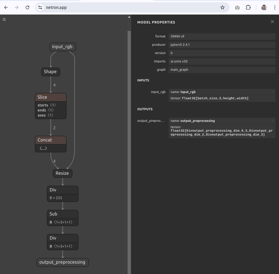
note
Note the name of the output node of the preprocessing.onnx model - output_preprocessing.
Next, let’s visualize the original eva02_large_patch14_448 model on Netron.
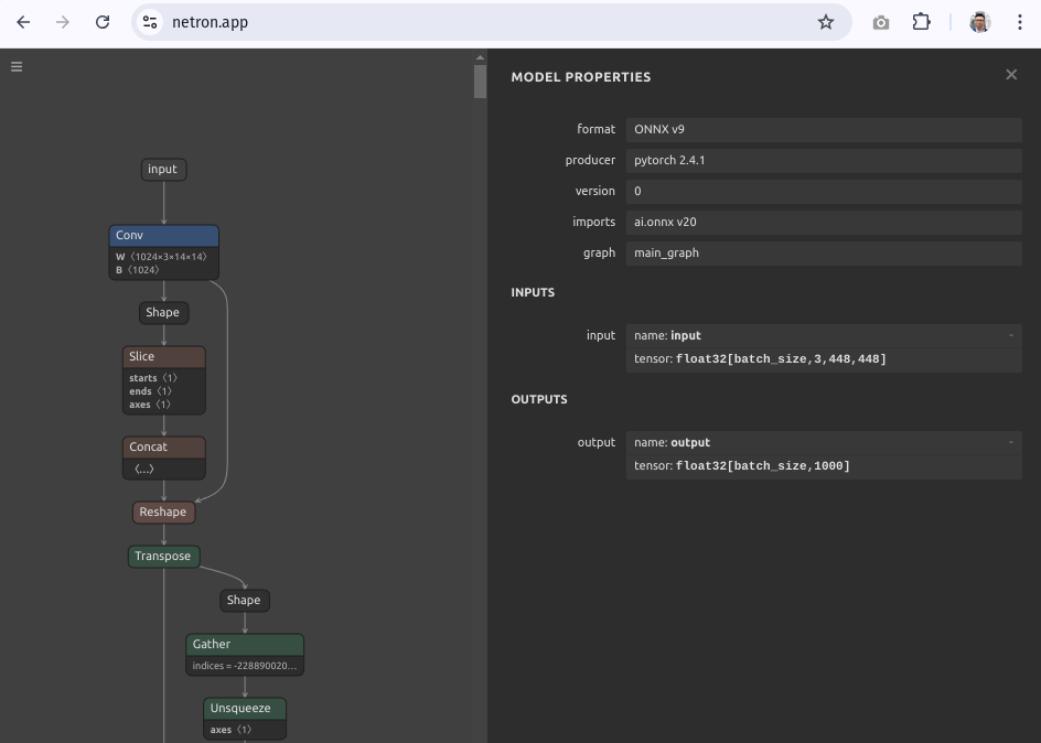
Note the name of the input node of the eva02_large_patch14_448 model. We will need this for the merge.
The name of the input node is input.
Now, we merge the preprocessing.onnx model with the eva02_large_patch14_448 model.
To achieve this, we need to merge the output of the preprocessing.onnx model with the input of the eva02_large_patch14_448 model.
To merge the models, we use the compose function from the onnx library.
import onnx

# Load the models
model1 = onnx.load("preprocessing.onnx")
model2 = onnx.load("eva02_large_patch14_448.onnx")

# Merge the models
merged_model = onnx.compose.merge_models(
    model1,
    model2,
    io_map=[("output_preprocessing", "input")],
    prefix1="preprocessing_",
    prefix2="model_",
    doc_string="Merged preprocessing and eva02_large_patch14_448 model",
    producer_name="dickson.neoh@gmail.com using onnx compose",
)

# Save the merged model
onnx.save(merged_model, "merged_model_compose.onnx")
Note the io_map parameter. This lets us map the output of the preprocessing model to the input of the original model. You must ensure that the input and output names of the models are correct.
If there are no errors, you will end up with a file called merged_model_compose.onnx in your working directory.
Let’s visualize the merged model on Netron.
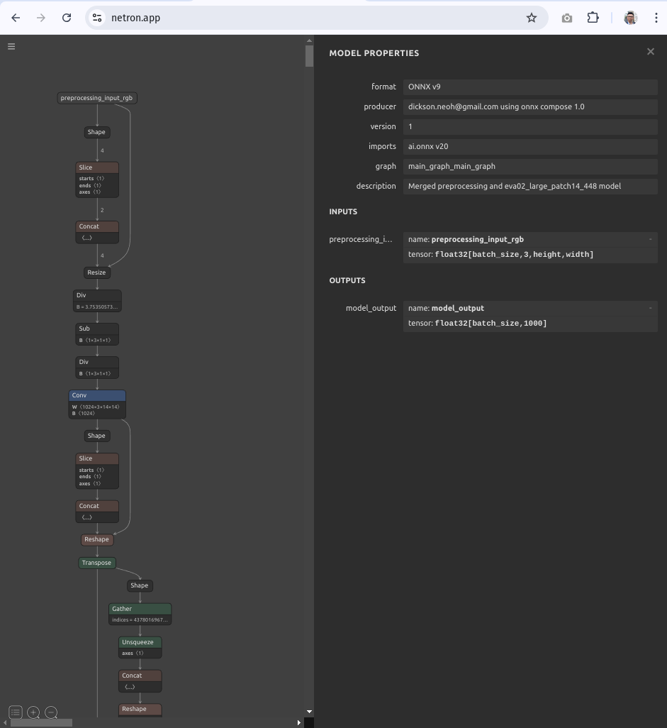
tip
The merged model expects an input of size [batch_size, 3, height, width].
This means that the model can take arbitrary input of size height, width and batch size.
Now using this merged model, let’s run the inference benchmark again using the TensorRT provider.
We’ll need to make a small change to how the input tensor is passed to the model.
def read_image(image: Image.Image):
    image = image.convert("RGB")
    img_numpy = np.array(image).astype(np.float32)
    img_numpy = img_numpy.transpose(2, 0, 1)
    img_numpy = np.expand_dims(img_numpy, axis=0)
    return img_numpy
Notice we are no longer doing the resize and normalization inside the function. This is because the merged model already includes these operations.
And the results are in!
- TensorRT with pre-processing: 12.875 ms per image, FPS: 77.67
That’s a 8x improvement over the original PyTorch model on the GPU and a whopping 123x improvement over the PyTorch model on the CPU! 🚀
Let’s do a final sanity check on the predictions.
- espresso: 34.48%
- cup: 2.16%
- chocolate sauce, chocolate syrup: 1.53%
- bakery, bakeshop, bakehouse: 1.01%
- eggnog: 0.98%
Looks like the predictions tally!
info
There are small value differences in the confidence values which is likely due to the precision difference between FP32 and FP16 and the normalization difference between the PyTorch model and the ONNX model.
🎮 Video Inference
Just for fun, let’s see how fast the merged model runs on a video.
The video inference code is also provided in the repo.
🚧 Conclusion
In this post we have seen how we can supercharge our TIMM models for faster inference using ONNX Runtime and TensorRT.
tip
In this post you’ve learned how to:
- 📥 Load any pre-trained model from TIMM
- 🔄 Convert the model to ONNX format
- 🖥️ Run inference with ONNX Runtime (CPU & GPU)
- 🎮 Run inference with TensorRT (GPU)
- 🛠️ Tweak the TensorRT parameters for better performance
- 🧠 Bake the pre-processing into the ONNX model
You can find the code for this post on my GitHub repository here.

Or simply check out the Hugging Face Spaces demo below.
note
There are other things that we’ve not explored in this post that will likely improve the inference speed. For example,
- Quantization - reducing the precision of the model weights from FP32 to FP8, INT8 or even lower.
- Pruning and Sparsity - removing the redundant components of the model to reduce the model size and improve the inference speed.
- Knowledge distillation - training a smaller and faster model to mimic the original model.
I will leave these as an exercise for the reader. And let me know if you’d like me to write a follow-up post on these topics.
Thank you for reading! I hope this has been helpful. If you’d like to find out how to deploy this model on Android check out the following post.

PyTorch at the Edge: Deploying Over 964 TIMM Models on Android with TorchScript and Flutter
- GitHub
- Scholar
- Telegram
🤟 Follow me
Don't want to miss any of my future content? Follow me on Twitter and LinkedIn where I share these tips in bite-size posts.
🔄 Share this post
❤️ Show some love
Creating free ML contents doesn't pay my bills. Support me in creating more free contents like these. Consider buying me a coffee. Your support means a lot to me.