Faster than GPU: How to 10x your Object Detection Model and Deploy on CPU at 50+ FPS


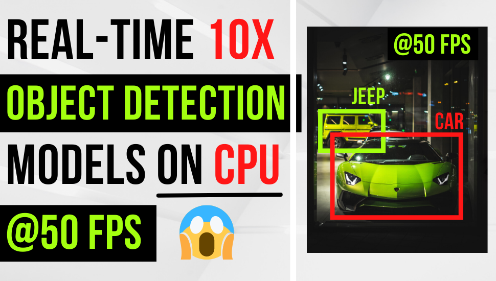
Table of Contents
🚦 Motivation
tip
By the end of this post, you will learn how to:
- Train state-of-the-art YOLOX model with your own data.
- Convert the YOLOX PyTorch model into ONNX and OpenVINO IR format.
- Run quantization algorithm to 10x your model’s inference speed.
P/S: The final model runs faster on the CPU than the GPU! 😱
Deep learning (DL), seems to be the magic word that makes anything mundane cool again. We find them everywhere - in news reports, blog posts, articles, research papers, advertisements, and even baby books.
Except in production 🤷♂️.
As much as we were made to believe DL is the answer to our problems, more than 85% of models don’t make it into production - according to a recent survey by Gartner.
The barrier? Deployment.
For some applications such as self-driving car, real-time deployment is critical and has huge implications.
As data scientists, even though we can easily train our models on GPUs, it is uncommon and sometimes impractical to deploy them on GPUs in production. On the other hand, CPUs are far more common in production environment, and a lot cheaper.
But can we feasibly deploy real-time DL models on a CPU? Running DL models on a CPU is orders of magnitude slower compared to GPU, right?
Wrong.
In this post, I will walk you through how we go from this 🐌🐌🐌
to this 🚀🚀🚀
Yes, that’s right, we can run DL models on a CPU at 50+ FPS 😱 and I’m going to show you how in this post. If that looks interesting, let’s dive in.
⛷ Modeling with YOLOX

We will use a state-of-the-art YOLOX model to detect the license plate of vehicles around the neighborhood. YOLOX is one of the most recent YOLO series models that is both lightweight and accurate.
It claims better performance than YOLOv4, YOLOv5, and EfficientDet models. Additionally, YOLOX is an anchor-free, one-stage detector which makes it faster than its counterparts.
Before we start training, let’s collect images of the license plates and annotate them. I collected about 40 images in total. 30 of the images will be used as the training set and 10 as the validation set.
tip
This is an incredibly small sample size for any DL model, but I found that it works reasonably well for our task at hand. We likely need more images to make this model more robust. However, this is still a good starting point.
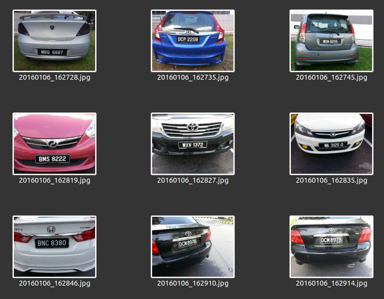
Sample images of vehicle license plates.
To label the images, let’s use the open-source CVAT labeling tool by Intel. There are a ton of other labeling tools out there feel free to use them if you are comfortable.
If you’d like to try CVAT, head to https://cvat.org/ - create an account and log in. No installation is needed.
A top menu bar should be visible as shown below.
Click on Task, fill in the name of the task, add related labels, and upload the images.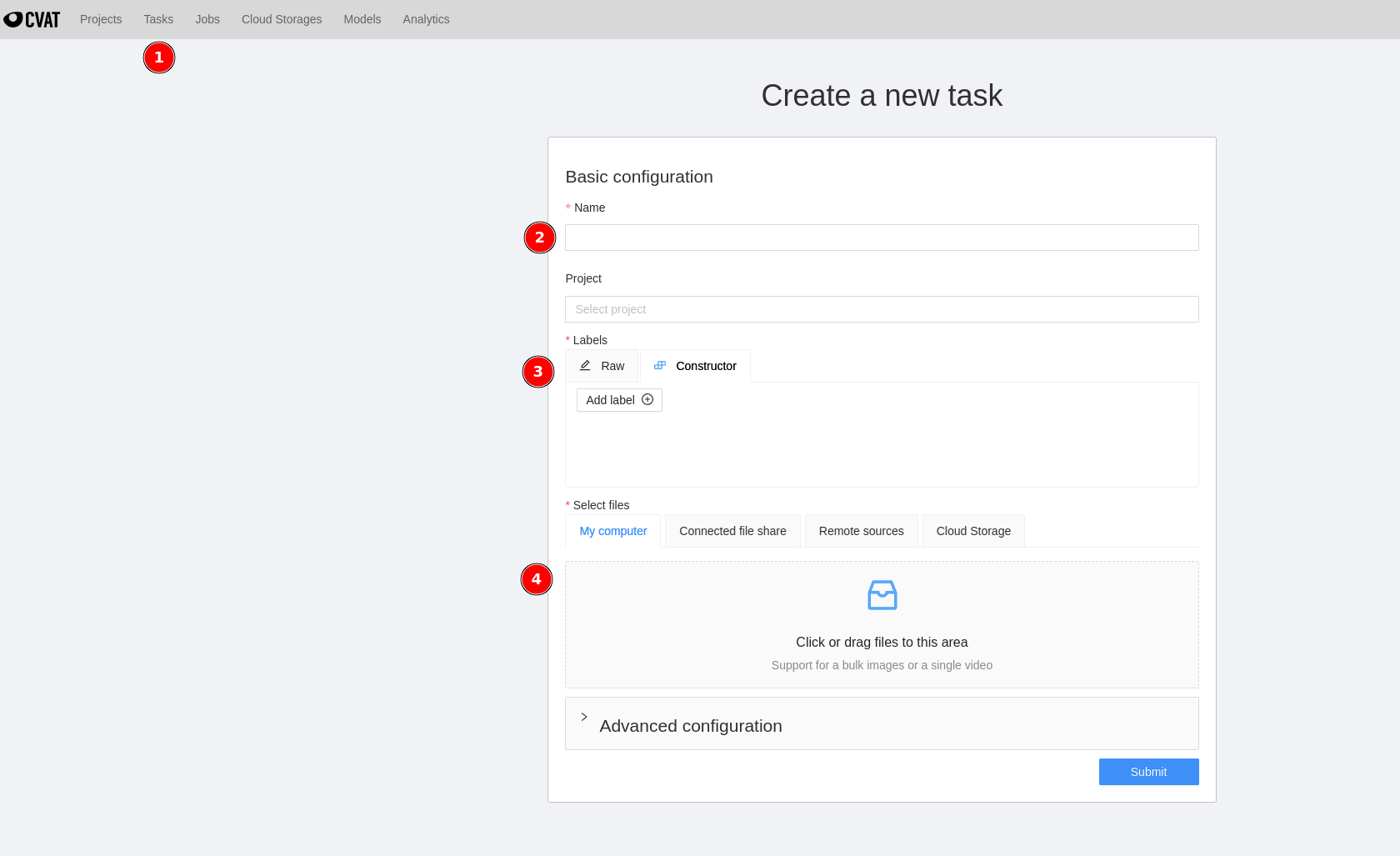
Since we are only interested in labeling the license plate, I’ve entered only one label - LP (license plate).
Once the uploading completes, you will see a summary page as below.
Click on Job #368378 at ③ and it should bring you to the labeling page.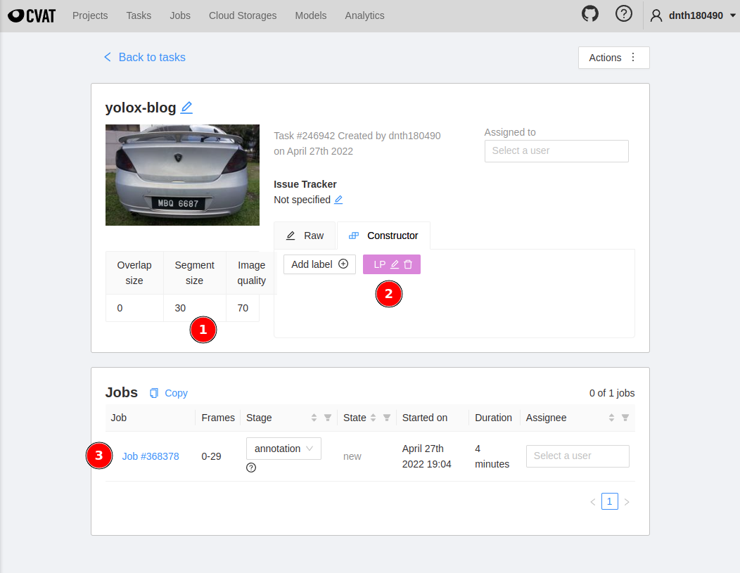
To start labeling, click on the square icon at ① and click Shape at ② in the figure below.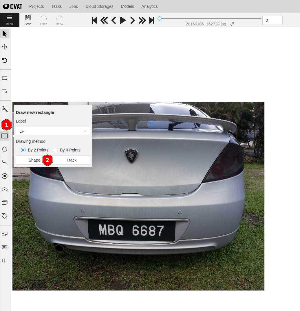
You can then start drawing bounding boxes around the license plate. Do this for all 40 images.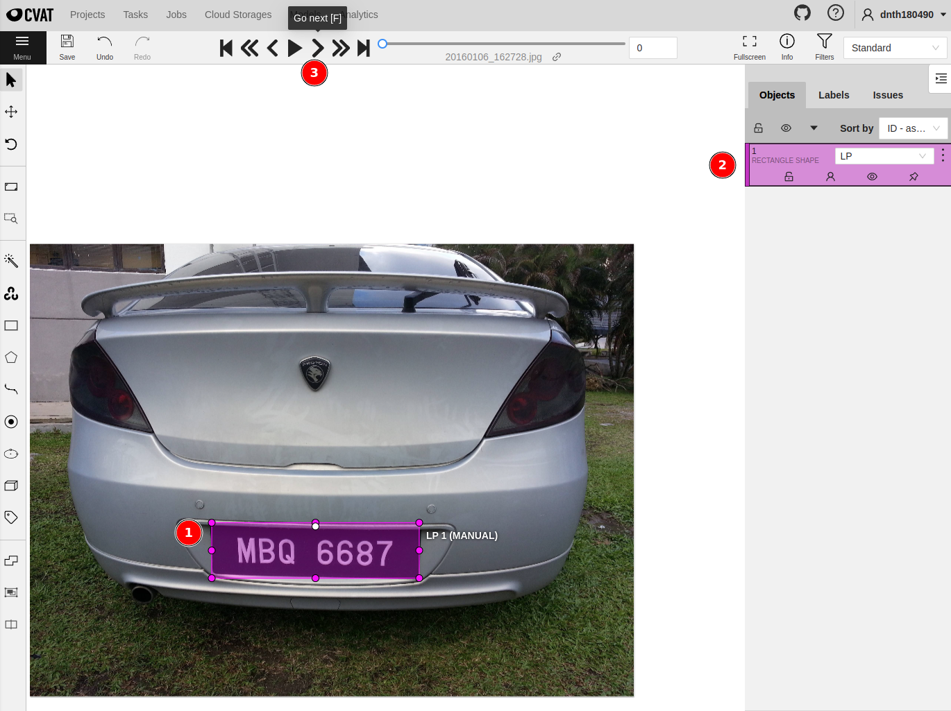
Once done, we are ready to export the annotations on the Tasks page.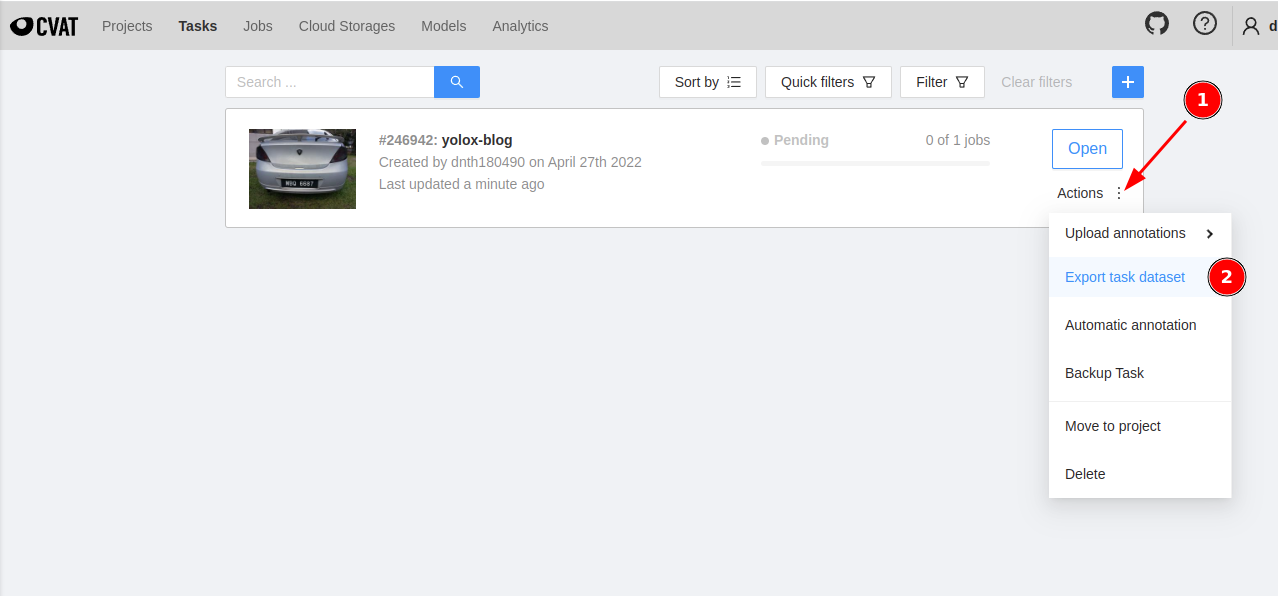
Make sure the format is COCO 1.0 and click on OK. If you’d like to download the images check the Save images box. Since I have those images already, I don’t have to download them.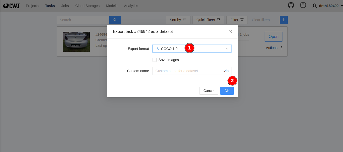
Now, that we have our dataset ready, let’s begin training. If you haven’t already, install the YOLOX package by following the instructions here.
Place your images and annotations in the datasets folder following the structure outlined here.
Next, we must prepare a custom Exp class.
The Exp class is a .py file where we configure everything about the model - dataset location, data augmentation, model architecture, and other training hyperparameters.
More info on the Exp class here.
For simplicity let’s use one of the smaller models - YOLOX-s.
There are other YOLOX models you can try like YOLOX-m, YOLOX-l, YOLOX-x, YOLOX-Nano, YOLOX-Tiny, etc.
Feel free to experiment with them.
More details are on the README of the YOLOX repo.
My custom Exp class for the YOLOX-s model looks like the following
| |
We are now ready to start training.
The training script is provided in the tools folder. To start training, run
python tools/train.py -f exps/example/custom/yolox_s.py -d 1 -b 64 --fp16 -o -c /path/to/yolox_s.pth
note
-fspecifies the location of the customExpfile.-dspecifies the number of GPUs available on your machine.-bspecifies the batch size.-cspecifies the path to save your checkpoint.--fp16tells the model to train in mixed precision mode.-ospecifies the option to occupy GPU memory first for training.
After the training completes, you can run inference on the model by utilizing the demo.py script in the same folder. Run
python tools/demo.py video -f exps/example/custom/yolox_s.py -c /path/to/your/yolox_s.pth --path /path/to/your/video --conf 0.25 --nms 0.45 --tsize 640 --device gpu
note
-fspecifies the path to the customExpfile.-cspecifies the path to your saved checkpoint.--pathspecifies the path to the video you want to infer on.--confspecifies the confidence threshold of the detection.--nmsspecifies the non-maximum suppression threshold.--tsizespecifies the test image size.--devicespecifies the device to run the model on -cpuorgpu.
I’m running this on a computer with an RTX3090 GPU. The output looks like the following.
Out of the box, the model averaged 40+ FPS on an RTX3090 GPU. But, on a Core i9-11900 CPU (a relatively powerful CPU to date) it averaged at 5+ FPS - not good for a real-time detection task.
Let’s improve that by optimizing the model.
🤖 ONNX Runtime

ONNX supports a cross-platform model accelerator known as the ONNX Runtime. This improves the inference performance of a wide variety of models capable of running on various operating systems.
Let’s convert our trained YOLOX-s model into the ONNX format.
For that, you must install the onnxruntime package via pip.
pip install onnxruntime
To convert our model run
python tools/export_onnx.py --output-name your_yolox.onnx -f exps/your_dir/your_yolox.py -c your_yolox.pth
Let’s load the ONNX model and run the inference using the ONNX Runtime.
As shown, the FPS slightly improved from 5+ FPS to about 10+ FPS with the ONNX model and Runtime on CPU - still not ideal for real-time inference. Just by converting the model to ONNX, we already 2x the inference performance.
Let’s see if we can improve that further.
🔗 OpenVINO Intermediate Representation
OpenVINO is a toolkit to optimize DL models. It enables a model to be optimized once and deployed on any supported Intel hardware including CPU, GPU, VPU, and FPGAs.
To optimize a model, we will use a tool known as Model Optimizer (MO) by Intel. MO converts all floating-point weights of the original model to FP16 data type.
The resulting form is known as the OpenVINO Intermediate Representation (IR) or called the compressed FP16 model. The compressed FP16 model takes half the disk space compared to the original model and may have some negligible accuracy drop.
Let’s convert our model into the IR form.
For that, we need to install the openvino-dev package.
pip install openvino-dev[onnx]==2022.1.0
Once installed, we can invoke the mo command to convert the model. mo is the abbreviation of
mo --input_model models/ONNX/yolox_s_lp.onnx --input_shape [1,3,640,640] --data_type FP16 --output_dir models/IR/
note
The mo accepts a few parameters:
--input_modelspecifies the path to the previously converted ONNX model.--input_shapespecifies the shape of the input image.--data_typespecifies the data type.--output_dirspecifies the directory to save the IR.
This results in a set of IR files that consists of an .xml and .bin file.
.xml- Describes the model architecture.bin- Contains the weights and biases of the model.
Together, you can deploy them on any of the supported Intel hardware.
Now, let’s run an inference using the IR files on the same video and observe its performance.
As you can see the FPS bumped up to 16+ FPS. It’s now beginning to look more feasible for real-time detection. Let’s call it a day and celebrate the success of our model! 🥳
Or, is there more to it? Enter 👇👇👇
🛠 Post-Training Quantization
Apart from the Model Optimizer, OpenVINO also comes with a Post-training Optimization Toolkit (POT) designed to supercharge the inference of DL models without retraining or finetuning.
To achieve that, POT runs 8-bit quantization algorithms and optimizes the model to use integer tensors instead of floating-point tensors on some operations. This results in a 2-4x faster and smaller model.
This is where the real magic happens.
From the OpenVINO documentation page, the POT supports two types of quantization:
DefaultQuantizationis a default method that provides fast and in most cases accurate results for 8-bit quantization.AccuracyAwareQuantizationenables remaining at a predefined range of accuracy drop after quantization at the cost of performance improvement. It may require more time for quantization.
The quantization algorithm requires a representative subset of the dataset to estimate the model accuracy during the quantization process. Let’s prepare a few images and put them in a separate directory.
We are going to use the DefaultQuantization in this post.
For that, let’s run
pot -q default -m models/IR/yolox_s_lp.xml -w models/IR/yolox_s_lp.bin --engine simplified --data-source data/pot_images --output-dir models/INT8
note
The pot command accepts a few parameters:
-mspecifies the directory to the.xmlfile.-wspecifies the directory to the.binfile.--enginespecifies the type of quantization algorithm.--data-sourcespecifies the directory of the images used to quantize the model.--output-dirspecifies the directory to save the quantized model.
This results in another set of IR files saved in --output-dir.
🚀 Real-time Inference @50+ FPS
Now, the moment of truth. Let’s load the quantized model and run the same inference again.
Boom!
The first time I saw the numbers, I could hardly believe my eyes. 50+ FPS on a CPU! That’s about 10x faster 🚀 compared to our initial model! Plus, this is also faster than the RTX3090 GPU!
Mind = blown 🤯
🏁 Conclusion
tip
In this post you’ve learned how to:
- Train a custom YOLOX model with your own dataset.
- Convert the trained model into ONNX and IR forms for inference.
- 10x the inference speed of the model with 8-bit quantization.
So, what’s next? To squeeze even more out of the model I recommend:
- Experiment with smaller YOLOX models like YOLOX-Nano or YOLOX-Tiny.
- Try using a smaller input resolution such as
416x416. We’ve used640x640in this post. - Try using the
AccuracyAwareQuantizationwhich runs quantization on the model with lesser accuracy loss.
There’s also a best practice guide to quantize your model with OpenVINO here.
If you enjoyed this post, you might also like the following post where I show how to accelerate your PyTorch Image Models (TIMM) 8x faster with ONNX Runtime and TensorRT.
Supercharge Your PyTorch Image Models: Bag of Tricks to 8x Faster Inference with ONNX Runtime & Optimizations
🙏 Comments & Feedback
I hope you’ve learned a thing or two from this blog post. If you have any questions, comments, or feedback, please leave them on the following Twitter/LinkedIn post or drop me a message.
Deploying object detection models on a CPU is a PAIN.
— Dickson Neoh 🚀 (@dicksonneoh7) May 3, 2022
In this thread I will show you how I optimized and 10x my YOLOX model from 5 FPS to 50 FPS on a CPU.
Yes!! CPU!
And yes for FREE.
The optimized model runs FASTER on a CPU than GPU 🤯 https://t.co/nlzjO8wmVV
A thread 👇
- GitHub
- Scholar
- Telegram
🤟 Follow me
Don't want to miss any of my future content? Follow me on Twitter and LinkedIn where I share these tips in bite-size posts.
🔄 Share this post
❤️ Show some love
Creating free ML contents doesn't pay my bills. Support me in creating more free contents like these. Consider buying me a coffee. Your support means a lot to me.