Squeezing the Best Performance Out of YOLOX with Weights and Biases


Table of Contents
🔎 Motivation
tip
By the end of this post you will learn how to:
- Install the Weights and Biases client and log the YOLOX training metrics.
- Compare training metrics on Weights and Biases dashboard.
- Picking the best model with mAP and FPS values.
“So many models, so little time!”
As a machine learning engineer, I often hear this phrase thrown around in many variations.
In object detection alone, there are already several hundreds of models out there. Within the YOLO series alone there are YOLOv1 to YOLOv5, YOLOR, YOLOP, YOLOS, PPYOLO, YOLOX, the list can go on forever.
With each passing day, better models are added as new discoveries are made. Which one do we pick? How do we know if it’s best for the application? If you’re new, this can easily get overwhelming.

In this post I will show you how I use a free tool known as Weights and Biases (Wandb) to quickly log your experiments and compare them side-by-side.
In the interest of time, we will limit our scope to the YOLOX series in this post. We will answer the following questions by the end of the post.
- How to keep track and log the performance of each model?
- How do the models compare to one another?
- How to pick the best model for your application?
In this blog post I will show you how I accomplish all of them by using Wandb.
PS: No Excel sheets involved 🤫
🕹 Wandb - Google Drive for Machine Learning
Life is short they say.
So why waste it on monitoring your deep learning models when you can automate them? This is what Wandb is trying to solve. It’s like Google Drive for machine learning.
Wandb helps individuals and teams build models faster. With just a few lines of code, you can compare models, log important metrics, and collaborate with teammates. It’s free to get started. Click here to create an account.

This post is a sequel to my previous post where I showed how to deploy YOLOX models on CPU at 50 FPS. This time around I will show you how I get the most from the YOLOX models by logging the performance metrics and comparing them on Wandb.
Let’s first install the Wandb client for Python:
pip install wandb
Next, run
wandb login
from your terminal to authenticate your machine. The API key is stored in ~/.netrc.
If the installation and authentication are completed successfully, you can now use Wandb to monitor and log all the YOLOX training metrics.
👀 Monitoring Training Metrics
Within the YOLOX series, there are at least 6 different variations of the model sorted from largest to smallest in size:
- YOLOX-X (largest)
- YOLOX-L
- YOLOX-M
- YOLOX-S
- YOLOX-Tiny
- YOLOX-Nano (smallest)
Let’s train all the YOLOX models and log the training metrics to Wandb. For that, you need to install the YOLOX library following the instructions here.
You’d also need to prepare a custom Exp file to specify the model and training hyperparameters.
I will use an existing Exp file from my last blog post.
All you need to do is run the train.py script from the YOLOX repository and specify wandb in the --logger argument.
python tools/train.py -f exps/example/custom/yolox_s.py \
                      -d 1 -b 64 --fp16 \
                      -o -c /path/to/yolox_s.pth \
                      --logger wandb \
                      wandb-project <your-project-name> \
                      wandb-id <your-run-id>
note
-fspecifies the location of the customExpfile.-dspecifies the number of GPUs available on your machine.-bspecifies the batch size.-cspecifies the path to save your checkpoint.--fp16tells the model to train in mixed precision mode.-ospecifies the option to occupy GPU memory first for training.--loggerspecifies the type of logger we want to use. Specifywandbhere.wandb-projectspecifies the name of the project on Wandb. (Optional)wandb-idspecifies the id of the run. (Optional)
If the optional arguments are not specified, a random project name and id will be generated. You can always change them on the Wandb dashboard later.
I’d recommend to specify self.save_history_ckpt = False in your Exp file.
If set to True this saves the model checkpoint at every epoch and uploads them to wandb.
This makes the logging process A LOT slower because every checkpoint is uploaded to wandb as an artifact.
Once everything is set in place, let’s run the training script and head to the project dashboard on Wandb to monitor the logged metrics.
After running the training for all the YOLOX models, the project dashboard should look like the following.
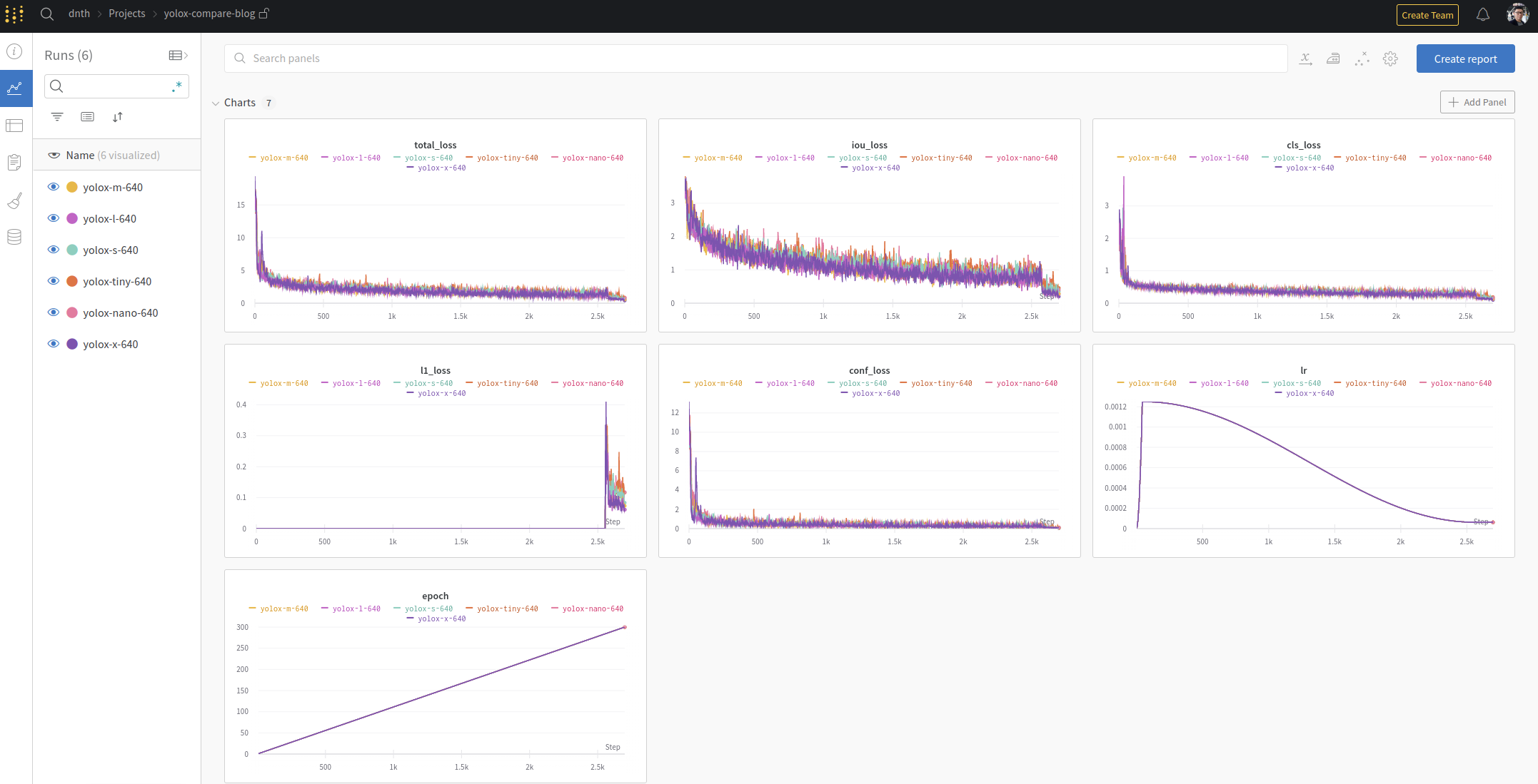
Logged metrics during training for all YOLOX models.
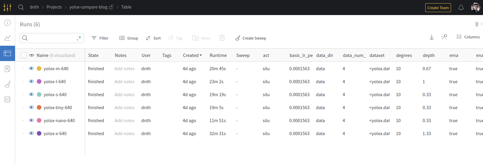
Logged hyperparameters for all YOLOX models.
As shown above, all the training metrics and hyperparameters are logged for each YOLOX model in an organized table.
You can share this dashboard with your teammates so they can view the metrics in real-time as you train.
You can also conveniently export the table and graphs into other forms such as .csv should you require.
I’m not a fan of Excel sheets, so I’ll keep them on Wandb 😎. Access my dashboard for this post here.
To gauge the quality of the model, we can look at the COCOAP50_95 plot or also known as the COCO Metric or mean average precision (mAP) plot.
The mAP plot indicates how well the model performs on the validation set (higher values are better) as we train the model and is shown below.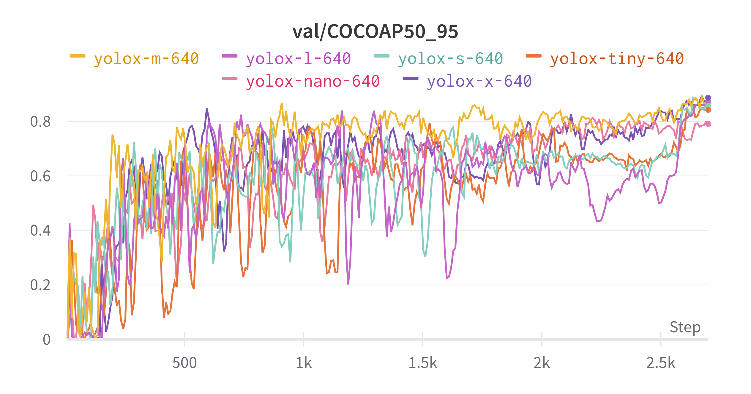
From the mAP plot, looks like YOLOX-X scored the highest mAP followed by YOLOX-L, YOLOX-M, YOLOX-S, YOLOX-Tiny and YOLOX-Nano.
It’s a little hard to tell from the figure above.
I encourage you to check out the dashboard where you can zoom in and resize the plots.
⚡️ Inference with Quantized Model
Comparing the mAP value on Wandb only gives us an idea of how well the model performs on the validation set. It does not indicate how fast the model will run in deployment and how well the model will perform in the real world.
In object detection, it is always good to verify the performance by visual inspection of the running model. For that, let’s run inference on a video for each model.
Running inference on a GPU is boring 🤷♂️, we know YOLOX models can run very fast on GPUs. To make it more interesting, let’s run the models on a CPU instead.
Traditionally, object detection models run slowly on a CPU. To overcome that, let’s convert the YOLOX models into a form that can run efficiently on CPUs.
For that, we use Intel’s Post-training Optimization Toolkit (POT) which runs an INT8 quantization algorithm on the YOLOX models.
Quantization optimizes the model to use integer tensors instead of floating-point tensors.
This results in a 2-4x faster and smaller models.
Plus, we can now run the models on a CPU for real-time inference!
If you’re new to my posts, I wrote on how to run the quantization here. Let’s check out how the models perform running on a Core i9 CPU 👇
YOLOX-X (mAP: 0.8869, FPS: 7+)
YOLOX-X is the largest model that scores the highest mAP. The PyTorch model is 792MB and the quantized model is about 100MB in size. The quantized YOLOX-X model runs only at about 7 FPS on a CPU.
YOLOX-L (mAP: 0.8729, FPS: 15+)
The PyTorch model is 434MB and the quantized model is about 56MB in size. The quantized YOLOX-L model runs at about 15 FPS on a CPU.
YOLOX-M (mAP: 0.8688, FPS: 25+)
The PyTorch model is 203MB and the quantized model is about 27MB. The quantized YOLOX-M model runs at about 25 FPS on a CPU.
YOLOX-S (mAP: 0.8560, FPS: 50+)
The PyTorch model is 72MB and the quantized model is about 10MB in size. The quantized YOLOX-S model runs at about 50 FPS on a CPU.
YOLOX-Tiny (mAP: 0.8422, FPS: 70+)
The PyTorch model is 41MB and the quantized model is about 6MB in size. The quantized YOLOX-Tiny model runs at about 70 FPS on a CPU.
YOLOX-Nano (mAP: 0.7905, FPS: 100+)
YOLOX-Nano scored the lowest on the mAP compared to others. The PyTorch model is 7.6MB and the quantized model is about 2MB in size. However, it is the fastest running model with over 100 FPS on CPU.
tip
- Larger models score higher mAP and lower FPS.
- Smaller models score lower mAP and higher FPS.
To answer the question of which model is best will ultimately depend on your application. If you need a fast model and only have a lightweight CPU on the edge, give YOLOX-Nano a try. If you prioritize accuracy over anything else and have a reasonably good CPU - YOLOX-X seems to fit.
Everything else lies in between.
This is a classic trade-off of accuracy vs latency in machine learning. Understanding your application well goes a long way to help you pick the best model.
⛳️ Wrapping up
tip
In this post we’ve covered
- How to install wandb client and use it with the YOLOX model.
- How to compare training metrics on the Wandb dashboard.
- Picking the best model using mAP values and inference speed on a CPU.
So, what’s next? In this short post, we have not explored all features available on Wandb. As the next steps, I encourage you to check the Wandb documentation page to see what’s possible.
Here are my 3 suggestions:
- Learn how to tune hyperparameters with Wandb Sweeps.
- Learn how to visualize and inspect your data on the Wandb dashboard.
- Learn how to version your model and data.
🙏 Comments & Feedback
I hope you’ve learned a thing or two from this blog post. If you have any questions, comments, or feedback, please leave them on the following Twitter/Linked post or drop me a message.
Picking an object detection model is a PAIN.
— Dickson Neoh 🚀 (@dicksonneoh7) May 11, 2022
Within the YOLO family there's YOLOv1 to YOLOv5, YOLOR, YOLOX, PPYOLO.. it's never ending 😵
How do you pick the right one for your application?
In this thread, I will show you how to squeze the best of YOLOX using @weights_biases pic.twitter.com/RjnmOz1mNh
- GitHub
- Scholar
- Telegram
🤟 Follow me
Don't want to miss any of my future content? Follow me on Twitter and LinkedIn where I share these tips in bite-size posts.
🔄 Share this post
❤️ Show some love
Creating free ML contents doesn't pay my bills. Support me in creating more free contents like these. Consider buying me a coffee. Your support means a lot to me.